
Numpy & Scipy - 1.9 Calculate Eigenvector and Eigenvalue of Matrix

Numpy & Scipy - 1.9 Calculate Eigenvector and Eigenvalue of Matrix
Numpy & Scipy 시리즈 (9 / 9)
- Numpy & Scipy - 1.1 Notation of Matrix and Vector, Matrix Input and Output
- Numpy & Scipy - 1.2 Convenient Functions of Matrix
- Numpy & Scipy - 1.3 Basic Manipulation of Matrices (1)
- Numpy & Scipy - 1.4 Basic Manipulation of Matrices (2)
- Numpy & Scipy - 1.5 Basic Manipulation of Matrices (3)
- Numpy & Scipy - 1.6 The Solution of Matrix Equation (General Matrices)
- Numpy & Scipy - 1.7 The Solution of Band Matrix
- Numpy & Scipy - 1.8 The Solution of Toeplitz Matrix and Circulant Matrix And How to Solve AX=B
- Numpy & Scipy - 1.9 Calculate Eigenvector and Eigenvalue of Matrix

일반 행렬의 eigenvalue 와 eigenvector
- $A\mathbf{x} = \lambda \mathbf{x}$ , $A\mathbf{x} = \lambda M \mathbf{x}$ 두 가지가 존재한다.
- eigenvalue 와 eigenvector 를 구하기 위해서는 linalg.eig 를 사용하면된다.
- eigvals 는 1D array (vector) 로 반환하고 $\lambda _1, \lambda _2, \dots, \lambda_n$
- eigvecs 는 2D array (matrix) 로 반환한다.
- eigvals 는 norm 이 큰 순서대로 정렬해서 나온다
1
2
3
4
5
6
7
A = np.array([[0, -1],[1, 0]], dtype=np.float64)

eigvals, eigvecs = linalg.eig(A)

prt(eigvals, fmt="%0.2f")
print()
prt(eigvecs, fmt="%0.2f")
1
2
3
4
( 0.00+1.00j), ( 0.00-1.00j)

( 0.71+0.00j), ( 0.71+0.00j)
( 0.00-0.71j), ( 0.00+0.71j)
- 또한 다음 eigenvector, eigenvalue 성질에서 알 수 있듯이
- \(A [\mathbf{v}_1 \; \mathbf{v}_2] = [\mathbf{v}_1 \; \mathbf{v}_2] \begin{bmatrix} \lambda_1 & 0 \\\ 0 & \lambda_2 \end{bmatrix} = [\lambda _1 \mathbf{v}_1 \; \lambda _2 \mathbf{v}_2]\) 임을 검증해보자.
1
2
3
4
5
6
7
comp1 = A @ eigvecs
comp2 = eigvecs @ np.diag(eigvals)
comp3 = eigvecs * eigvals

print(np.allclose(comp1, comp2))
print(np.allclose(comp2, comp3))
print(np.allclose(comp1, comp3))
1
2
3
True
True
True
- 2D array 인 eigvecs $\begin{bmatrix} 1 & 1 \\ -i & i \end{bmatrix}$ 에서 슬라이싱을 통해 $\mathbf{v}_1, \mathbf{v}_2$ 를 뽑아낼 수도 있다.
1
2
3
4
5
6
v1 = eigvecs[:, 0]
v2 = eigvecs[:, 1]

prt(v1, fmt="%0.2f")
print()
prt(v2, fmt="%0.2f")
1
2
3
( 0.71+0.00j), ( 0.00-0.71j)

( 0.71+0.00j), ( 0.00+0.71j)
- 또한 $A\mathbf{v}_1 = \lambda _1 \mathbf{v}_1$ 을 다음과 같이 표현할 수 있다.
1
eigvals[0] * eigvecs[:, 0]
일반 행렬의 eigenvalue만 구하기
- 행렬 A의 사이즈와 A의 eigenvector 사이즈의 크기는 같다. 따라서 linalg.eig 로 eigenvector 까지 구하려면 work-load 부담이 커진다.
- 따라서 eigenvector 를 따로 계산하지 않는 방법을 선호한다.
1
2
3
4
A = np.array([[0, -1],[1, 0]], dtype=np.float64)

eigvals = linalg.eig(A, right=False)
prt(eigvals, fmt="%0.2f")
1
( 0.00+1.00j), ( 0.00-1.00j)
Symmetric or Hermitian 행렬의 eigenvalue, eigenvector
- $A\mathbf{x} = \lambda \mathbf{x}$ 모두 실수이고 symmetric, hermitian 만 가능하다.
- $A\mathbf{x} = \lambda M \mathbf{x}$ 는 positive definite 만 가능
- linalg.eigh 를 사용하며 알고리즘은
- reduction to tridiagonal form, householder
- dqds algorithm, relatively robust representations -> python 에서 실제로 사용하는 알고리즘 더 효율적임
1
2
3
4
5
6
7
8
9
10
11
12
A = np.array([[6,3,1,5],[3,0,5,1],[1,5,6,2],[5,1,2,2]], dtype=np.float64)

eigvals, eigvecs = linalg.eigh(A) # eigvals 정렬이 norm 크기순으로는 제대로 안됨

prt(eigvals, fmt="%0.2f")
print()
prt(eigvecs, fmt="%0.2f")

comp1 = A@eigvecs
comp2 = eigvecs * eigvals

print(np.allclose(comp1, comp2))
1
2
3
4
5
6
7
8
9
10
11
# eigenvalues
-3.75, -0.76,  6.09,  12.42

# eigenvector
 0.36, -0.41,  0.58,  0.61
-0.76, -0.44, -0.25,  0.40
 0.42,  0.15, -0.71,  0.54
-0.33,  0.78,  0.30,  0.43

# 검증
True
- eigenvector 를 구할 필요없을때
1
eigvals = linalg.eigh(A, M, eigvals_only=True) # 로 하면됨
계산 시간 측정 방법
- timeit.default_timer() 를 통해 프로그램 시간 측정이 가능하다.
1
2
3
4
5
6
7
import timeit

start = timeit.default_timer()
eigvals = linalg.eigh(A, eigvals_only=True)
end = timeit.default_timer()
computing_time = end - start
print(computing_time)
1
2.3082999999979315e-05
- eig 와 eigh 계산 속도 비교
- eig : 21.69 s , eigh : 5,45 s
- 역시 symmetric 행렬을 계산하는 속도가 월등히 빠르다..
선형대수학개론에서 배운 QR Algorithm 은 못쓰는걸까?
- scipy 에선 low level lapack function 을 사용하여 QR Algorithm 으로 사용할 수 있지만..
- 하지만 scipy eigh 5.45s, 강좌 커스텀함수 eigh 9.54s 걸려서 검증된 scipy 사용하자!
Example 1.
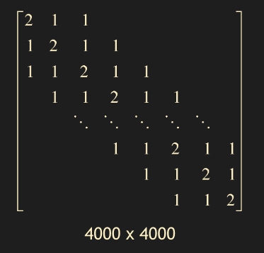
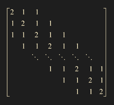
1000x1000 matrix 생성
eig 와 eigh 를 활용하여 eigenvalue 와 eigenvector 를 구하고 타당성 검증하기
import timeit 을 사용하여 계산 시간 비교하기
1
2
3
4
5
6
7
8
9
10
11
12
13
14
15
16
17
18
19
20
21
22
23
24
25
26
27
28
29
30
31
32
33
34
35
import numpy as np
from scipy import linalg
import timeit
from print_lecture import print_custom as prt

n = 1000

band1 = 2 * np.ones((n,), dtype=np.float64) # k = 0
band2 = np.ones((n-1), dtype=np.float64)    # k = 1
band3 = np.ones((n-2), dtype=np.float64)    # k = 2

b = np.ones((n,), dtype=np.float64)

A_full = np.diag(band1) + np.diag(band2, k=1) + np.diag(band3, k=2) + np.diag(band2, k=-1) + np.diag(band3, k=-2)

#print(A_full)

eig_start_time = timeit.default_timer()
eigvals1, eigvecs1 = linalg.eig(A_full)
eig_end_time = timeit.default_timer()
eig_computing_time = eig_end_time - eig_start_time

eigh_start_time = timeit.default_timer()
eigvals2, eigvecs2 = linalg.eigh(A_full)
eigh_end_time = timeit.default_timer()
eigh_computing_time = eigh_end_time - eigh_start_time

# 타당성 검증
print(np.allclose(A_full@eigvecs1, eigvals1*eigvecs1))
print(np.allclose(A_full@eigvecs2, eigvals2*eigvecs2))

# 계산 시간 비교
print(f"eig computing time : {eig_computing_time}")
print(f"eigh computing time : {eigh_computing_time}")
이 기사는 저작권자의 CC BY 4.0 라이센스를 따릅니다.