
Numpy & Scipy - 1.4 Basic Manipulation of Matrices (2)

- Numpy & Scipy - 1.1 Notation of Matrix and Vector, Matrix Input and Output
- Numpy & Scipy - 1.2 Convenient Functions of Matrix
- Numpy & Scipy - 1.3 Basic Manipulation of Matrices (1)
- Numpy & Scipy - 1.4 Basic Manipulation of Matrices (2)
- Numpy & Scipy - 1.5 Basic Manipulation of Matrices (3)
- Numpy & Scipy - 1.6 The Solution of Matrix Equation (General Matrices)
- Numpy & Scipy - 1.7 The Solution of Band Matrix
- Numpy & Scipy - 1.8 The Solution of Toeplitz Matrix and Circulant Matrix And How to Solve AX=B
- Numpy & Scipy - 1.9 Calculate Eigenvector and Eigenvalue of Matrix

hstack / vstack
- np.hstack((tuple)), np.vstack((tuple)) : 2D array, 1D array, 두 개가 혼합된 형태로 조합이 가능하다.
- 둘 다 deep copy 이다.
(1) 2D array 인 경우
2x3 2x2 hstack
1
2
3
4
5
6
7
8
9
10
a = np.array([[1,2,3], [4,5,6]], dtype=np.float64)
b = np.array([[-1,-2], [-3,-4]], dtype=np.float64)

new_mat = np.hstack( (a,b) ) # 입력 시 tuple 형태임에 주의

new_mat = np.hstack( (a,b,b,b) ) # 여러개 조합 가능

prt(new_mat, fmt="%0.1f", delimiter=",")
print()
print(new_mat.shape)
1
2
3
4
5
6
# 수평으로 행렬이 조합이 된 것을 확인할 수 있다.
1.0, 2.0, 3.0,-1.0,-2.0
4.0, 5.0, 6.0,-3.0,-4.0

# 2x5 matrix
(2, 5)
- 3x3 2x2 hstack
1
2
3
4
5
6
7
8
a = np.array([[1,2,3],[4,5,6]], dtype=np.float64)
b = np.array([[-1,-2,-3],[-4,-5,-6],[-7,-8,-9]], dtype=np.float64)

new_mat = np.hstack( (a,b) ) # 입력 시 tuple 형태임에 주의

prt(new_mat, fmt="%0.1f", delimiter=",")
print()
print(new_mat.shape)
1
2
# 2x3 3x3 는 2row 와 3row hstack 조합이 불가능
ValueError: all the input array dimensions except for the concatenation axis must match exactly, but along dimension 0, the array at index 0 has size 2 and the array at index 1 has size 3
- 2x3 2x2 vstack
1
2
3
4
5
6
7
8
a = np.array([[1,2,3], [4,5,6]], dtype=np.float64)
b = np.array([[-1,-2], [-3,-4]], dtype=np.float64)

new_mat = np.vstack( (a,b) ) # 입력 시 tuple 형태임에 주의

prt(new_mat, fmt="%0.1f", delimiter=",")
print()
print(new_mat.shape)
1
2
3
# 2x3 2x2 는 vstack 조합이 안되기 때문에 다음과 같은 에러가 발생한다.

ValueError: all the input array dimensions except for the concatenation axis must match exactly, but along dimension 1, the array at index 0 has size 3 and the array at index 1 has size 2
- 2x3 3x3 vstack
1
2
3
4
5
6
7
8
a = np.array([[1,2,3],[4,5,6]], dtype=np.float64)
b = np.array([[-1,-2,-3],[-4,-5,-6],[-7,-8,-9]], dtype=np.float64)

new_mat = np.vstack( (a,b) ) # 입력 시 tuple 형태임에 주의

prt(new_mat, fmt="%0.1f", delimiter=",")
print()
print(new_mat.shape)
1
2
3
4
5
6
7
1.0, 2.0, 3.0
4.0, 5.0, 6.0
-1.0,-2.0,-3.0
-4.0,-5.0,-6.0
-7.0,-8.0,-9.0

(5, 3)
(2) 1D array 인 경우
- hstack
- 1D array 벡터가 더 길어진다.
1
2
3
4
5
6
7
8
a = np.array([1,2,3], dtype=np.float64)
b = np.array([4,5,6], dtype=np.float64)

new_mat = np.hstack( (a,b) ) # 입력 시 tuple 형태임에 주의

prt(new_mat, fmt="%0.1f", delimiter=",")
print()
print(new_mat.shape)
1
2
3
1.0, 2.0, 3.0, 4.0, 5.0, 6.0

(6,)
- vstack
- 행렬이 만들어진다.
1
2
3
4
5
6
7
8
a = np.array([1,2,3], dtype=np.float64)
b = np.array([4,5,6], dtype=np.float64)

new_mat = np.vstack( (a,b) ) # 입력 시 tuple 형태임에 주의

prt(new_mat, fmt="%0.1f", delimiter=",")
print()
print(new_mat.shape)
1
2
3
4
1.0, 2.0, 3.0
4.0, 5.0, 6.0

(2, 3)
(3) 2D array 와 1D array 혼합된 형태
- hstack
- hstack 은 무조건 에러가 발생한다. 혼합된 형태는 vstack 만 된다.
1
2
3
4
5
6
7
8
a = np.array([[1,2,3],[4,5,6]],dtype=np.float64)
b = np.array([7,8,9], dtype=np.float64)

new_mat = np.hstack( (a,b) ) # 입력 시 tuple 형태임에 주의

prt(new_mat, fmt="%0.1f", delimiter=",")
print()
print(new_mat.shape)
1
ValueError: all the input arrays must have same number of dimensions, but the array at index 0 has 2 dimension(s) and the array at index 1 has 1 dimension(s)
- vstack
- 2x3 2D array 와 1x3 1D array 를 조합
1
2
3
4
5
6
7
8
a = np.array([[1,2,3],[4,5,6]],dtype=np.float64)
b = np.array([7,8,9], dtype=np.float64)

new_mat = np.vstack( (a,b) ) # 입력 시 tuple 형태임에 주의

prt(new_mat, fmt="%0.1f", delimiter=",")
print()
print(new_mat.shape)
1
2
3
4
5
1.0, 2.0, 3.0
4.0, 5.0, 6.0
7.0, 8.0, 9.0

(3, 3)
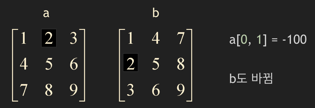
transpose method
- 말 그대로 행렬을 transpose 전치 하는 함수
swallow copy 이다.
- (1) transpose property
1
2
3
4
5
6
7
c = np.array([[1,2,3],[4,5,6],[7,8,9]], dtype=np.float64)

d = c.T

prt(c, fmt="%0.1f", delimiter=",")
print()
prt(d, fmt="%0.1f", delimiter=",")
1
2
3
4
5
6
7
8
9
# c matrix
1.0, 2.0, 3.0
4.0, 5.0, 6.0
7.0, 8.0, 9.0

# d matrix (transpose of c)
1.0, 4.0, 7.0
2.0, 5.0, 8.0
3.0, 6.0, 9.0
- swallow copy 예시
(2) transpose method
1D array 를 transpose() 하면 그대로 1D array 로 나온다.
1
2
3
4
5
6
7
8
9
10
11
e = np.array([1,2,3], dtype=np.float64)

f = e.transpose()

g = np.copy(e.transpose()) # np.copy 를 통해 deep copy 가 가능

prt(e, fmt="%0.1f", delimiter=",")
print(e.shape)
print()
prt(f, fmt="%0.1f", delimiter=",")
print(f.shape)
1
2
3
4
5
1.0, 2.0, 3.0
(3,)

1.0, 2.0, 3.0
(3,)
real / imag / conjugate
- real, imag 는 각 행렬 entry 들의 실수 부분, 허수 부분을 가져와서 반환한다.
- imag 의 경우 허수 부분을 가져와서 실수 행렬 or 벡터를 반환한다.
둘 다 swallow copy 이다.
- conjugate 는 deep copy 이다.
1
2
3
4
5
6
7
8
9
10
11
12
13
14
15
16
17
18
19
20
21
a = np.array([[1-2j, 3+1j, 1], [1+2j, 2-1j, 7]], dtype=np.complex128)

a_real = r.real

# prt(a, fmt="%0.1f", delimiter=",")
# print()
# prt(a_real, fmt="%0.1f", delimiter=",")

a_imag = r.imag # 허수부분을 실수로 반환하는것임ㅇ

# prt(a, fmt="%0.1f", delimiter=",")
# print()
# prt(a_imag, fmt="%0.1f", delimiter=",")


a_conj = r.conjugate() # conjugate 을 취하면 허수부분에 - 곱해져서 나옴
# deep copy

# prt(a, fmt="%0.1f", delimiter=",")
# print()
# prt(a_conj, fmt="%0.1f", delimiter=","
1
2
3
4
5
6
7
8
9
10
11
12
13
14
15
# a matrix
( 1.0-2.0j),( 3.0+1.0j),( 1.0+0.0j)
( 1.0+2.0j),( 2.0-1.0j),( 7.0+0.0j)

# real
1.0, 3.0, 1.0
1.0, 2.0, 7.0

# imag
-2.0, 1.0, 0.0
 2.0,-1.0, 0.0

# conjugate
( 1.0+2.0j),( 3.0-1.0j),( 1.0+0.0j)
( 1.0-2.0j),( 2.0+1.0j),( 7.0+0.0j)
Multiplication
- Scalar Multiplication
- 순서가 상관이 없음 result = r * A = A * r
1
2
3
4
5
6
7
8
A = np.array([[1,2,1],[2,1,3],[1,3,1]], dtype=np.float64)
scalar = 5.0

result = scalar * A

prt(A, fmt="%0.1f", delimiter=",")
print()
prt(result, fmt="%0.1f", delimiter=",")
1
2
3
4
5
6
7
1.0, 2.0, 1.0
2.0, 1.0, 3.0
1.0, 3.0, 1.0

5.0, 10.0, 5.0
10.0, 5.0, 15.0
5.0, 15.0, 5.0
- Matrix Mutliplication
순서가 매우 중요함 수학적 행렬 곱셈과 똑같음
- ”@” operator 를 사용하는 방법과
- np.matmul() 함수가 존재한다.
1
2
3
4
5
6
7
8
9
10
11
12
13
14

A = np.array([[1,2,3], [3,2,1]], dtype=np.float64)
B = np.array([[2,1],[1,2],[-3, 3]], dtype=np.float64)

result = A @ B
result2 = np.matmul(A, B)

prt(A, fmt="%0.1f", delimiter=",")
print()
prt(B, fmt="%0.1f", delimiter=",")
print()
prt(result, fmt="%0.1f", delimiter=",")
print()
prt(result2, fmt="%0.1f", delimiter=",")
1
2
3
4
5
6
7
8
9
10
11
12
13
14
1.0, 2.0, 3.0
3.0, 2.0, 1.0

2.0, 1.0
1.0, 2.0
-3.0, 3.0

# A @ B
-5.0, 14.0
 5.0, 10.0

# np.matmul(A,B)
-5.0, 14.0
 5.0, 10.0
- Matrix-Vector Multiplication
- 마찬가지로 result = A @ u , result = np.matmul(A,u) 를 사용해서 계산이 가능하다.
- dot product 아니다!
1
2
3
4
5
6
7
8
9
10
A = np.array([[1,2,1],[2,1,3],[1,3,1]], dtype=np.float64)
u = np.array([5,1,3], dtype=np.float64)

Au = np.matmul(A, u)

prt(A, fmt="%0.1f", delimiter=",")
print()
prt(u, fmt="%0.1f", delimiter=",")
print()
prt(Au, fmt="%0.1f", delimiter=",")
1
2
3
4
5
6
7
1.0, 2.0, 1.0
2.0, 1.0, 3.0
1.0, 3.0, 1.0

5.0, 1.0, 3.0

10.0, 20.0, 11.0
Inner Product : vdot
- result = np.vdot(u, v)
여기서 u, v 는 벡터이다.
- Inner Product 를 진행하면 다음과 같이 linear combination 형태로 표현된다.
real vector : $\quad \mathbf{u} \cdot \mathbf{v} = u_1v_1 + u_2v_2 + \dots + u_nv_n$
complex vector : $ \quad \mathbf{u} \cdot \mathbf{v} = u_1\bar{v}_1 + u_2\bar{v}_2 + \dots + u_n\bar{v}_n = \bar{u_1v_1} + \bar{u_2v_2} + \dots + \bar{u_nv_n}$
- 예시..
1
2
3
4
5
6
7
8
9
10
u = np.array([1,1,1,1], dtype=np.float64)
v = np.array([-1,1,-1,1], dtype=np.float64)

vdot = np.vdot(u,v)

prt(u, fmt="%0.1f", delimiter=",")
print()
prt(v, fmt="%0.1f", delimiter=",")
print()
print(vdot)
1
2
3
4
5
 1.0, 1.0, 1.0, 1.0

-1.0, 1.0,-1.0, 1.0

0.0
Norm
- 우리가 이전까지 선형대수학에서 배운 벡터의 norm 은 \(\lVert \mathbf{x} \rVert _2 = \left( \sum_{i=1}^n x_i^2 \right)^{1/2} \quad l_2 \mbox{-vector norm (Euclidean)}\) 이런 식으로 정의 했었고 이는 $l_2$ norm 이라고 부른다. 이외에도 많은 벡터 norm 들이 존재한다.
vector norm
\[\lVert \mathbf{x} \rVert _1 = \sum_{i=1}^n \lvert x_i \rvert \quad l_1 \mbox{-vector norm}\] \[\lVert \mathbf{x} \rVert _2 = (\sum_{i=1}^n \lvert x_i^2 \rvert)^{1/2} \quad l_2 \mbox{-vector norm (Euclidean)}\] \[\lVert \mathbf{x} \rVert _{\infty} = \max_{1 \le i \le n} \lvert x_i \rvert\]
- 그리고 마찬가지로 행렬의 norm 역시 존재하는데, 벡터 norm 과 같이 $l_1, l_2, l_{\infty}$ norm 이 존재한다.
matrix norm
\[\lVert A \rVert _1 = \max_{1 \le j \le n} \sum_{i=1}^m \lvert a_{ij} \rvert \quad l_1 \mbox{-matrix norm}\] \[\lVert A \rVert _2 = \sigma _{\max} \le \left( \sum_{i=1}^m \sum_{j=1}^n \lvert a_{ij} \rvert ^2 \right)^{1/2} \quad l_2 \mbox{-matrix norm (spectral)}\] \[\lVert A \rVert _{\infty} = \max_{1 \le i \le m} \sum_{j=1}^n \lvert a_{ij} \rvert \quad l_{\infty} \mbox{-matrix norm}\]
- numpy 에서 이 linalg.norm 을 사용하여 구하려면 scipy 라이브러리를 사용해야한다.
1
from scipy import linalg
- 예시
1
2
3
4
5
6
7
w = np.array([1,1], dtype=np.float64)

norm = linalg.norm(w, 2)

prt(w, fmt="%0.1f", delimiter=",")
print()
print(norm)
1
2
3
 1.0, 1.0

 1.4142135623730951
- 또한 $l_{\infty}$ norm 을 구하려면 inf 를 매개변수로 집어넣으면 된다.
1
norm = linalg.norm(a, 2, inf)
slicing - 행렬 혹은 벡터의 일부만 뽑아내기
swallow copy 이다.
예시
1
2
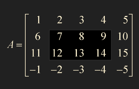
A = np.array([[1,2,3,4,5], [6,7,8,9,10], [11,12,13,14,15], [-1,-2,-3,-4,-5]])
sub_A = A[1:3, 1:4]
- row : 1~2, column : 1~3 을 가져오겠다는 뜻이다.
- 즉 : 뒤에 있는 인덱스 -1 까지 가져오겠다는 뜻이다!
- 1:3 을 입력하면 실제로는 1:2 까지 가져옴
1
2
3
4
5
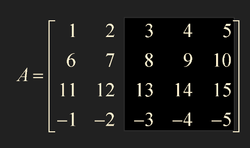
sub_A = A[0:5, 2:6]
# 다음과 동일하다
sub_A = A[ : , 2: ]
- : 는 처음부터 끝까지
- 2: 는 2 뒤로 전부
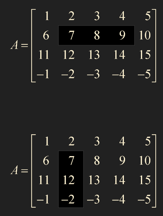
- row, column 쪽에 slicing operator : 를 붙이지 않으면 1D array 로 반환한다.
- np.reshape 를 통해 2D array 로 변환할 수 있다.
1
2
3
4
5
6
7
sub_A1 = A[1:2, 1:4] # 2D array 로 반환
sub_A2 = A[1, 1:4] # 1D array 로 반환

sub_A3 = A[1: , 1:2] #2D array 로 반환
sub_A4 = A[1:, 1] #1D araay 로 반환

sub_A5 = np.reshape(sub_A3, (3,1)) # 1D array -> 2D array
1
2
3
4
5
6
7
8
9
10
11
12
13
14
15
16
17
18
19
20
21
22
23
#sub_A1
7.0, 8.0, 9.0
(1, 3)

#sub_A2
7.0, 8.0, 9.0
(3,)

#sub_A3
 7.0
 12.0
-2.0
(3, 1)

#sub_A4
7.0, 12.0,-2.0
(3,)

#sub_A5
 7.0
 12.0
-2.0
(3, 1)
Example 1.
$A = \begin{bmatrix} 1 & 2 \\ 3 & 4 \end{bmatrix} \quad \mathbf{x} = \begin{bmatrix} 5 \\ 6 \end{bmatrix} $
$A, \mathbf{x}$ 를 각각 변수에 담아 2D,1D array 로 저장하고 1D array 는 transpose 가 안됨을 감안하여 quadratic form 인 $\mathbf{x}^TA\mathbf{x}$ 를 구해보기.
1) 2D array 로 변환해보기 (np.reshape)
2) np.vdot 사용해보기
1
2
3
4
5
6
7
8
9
10
11
12
13
14
15
16
17
18
19
20
import numpy as np
from print_lecture import print_custom as prt
from scipy import linalg

A = np.array([[1,2],[3,4]], dtype=np.float64)
x = np.array([5,6], dtype=np.float64)

# 1)
x_t = np.reshape(x, (2,1))

result1 = np.matmul(np.matmul(x_t.T, A), x)

print(result1)

# 2) np.vdot

result2 = np.vdot(x, A @ x)

print(result2)
1
2
3
4
5
6
7

# 1번 결과
319.0

# 2번 결과
319.0