
Machine Learning - Multiple Linear Regression

Machine Learning - Multiple Linear Regression
Supervised Machine Learning 시리즈 (6 / 7)
TL;DR — 핵심 요약
- 다중 선형 회귀는 여러 특성(feature)을 동시에 사용해 출력값을 예측하는 알고리즘이다
- Vectorization을 활용하면 코드가 간결해지고 NumPy/GPU 병렬 연산으로 속도가 향상된다
- dot product(내적)로 w⃗·x⃗를 계산하면 반복문 없이 모든 특성을 한 번에 처리할 수 있다
- 경사 하강법(Gradient Descent)은 다중 파라미터에서도 동일한 방식으로 적용된다

해당 포스트는 Andrew Ng 교수님의 Machine Learning Specialization 특화 과정에 대한 정리 내용을 참고하였습니다.
목차
Vectorization
Python Numpy 실습
Gradient Descent With Multiple Variables
Vectorization - 벡터화
- Vectorization 을 사용하여 학습 알고리즘을 구현할 때, 코드를 더 간결하게 작성가능하고 실행 속도도 향상된다. 또한 현대적인 수치선형대수학 라이브러리를 사용 가능하며 GPU 하드웨어를 가속화 하기 위한 코드를 작성하기도 한다.
Parameters and features
- Vectorziation 을 적용하지 않은 방법으로 계산 해보자.
1
2
3
w = np.array([1.0, 2.5, -3.3])
b = 4
x = np.array([10,20,30])
Without Vectorization 1
- 모델의 예측
1
2
3
f = w[0] * x[0] +
    w[1] * x[1] +
    w[2] * x[2] + b
- 이런 방법은 $n = 100000$ 까지 가면 매우 비효율적임..
Without Vectorization 2
- 따라서 그나마 효율적인 for 문을 돌려보면..
1
2
3
4
f = 0
for j in range(0, n):
    f = f + w[j] * x[j]
f = f + b
Vectorization
- Numpy 라이브러리를 사용하여 Vectorization 을 해보면 다음과 같다.
1
f = np.dot(w,x) + b
- np.dot 함수는 컴퓨터의 병렬 하드웨어를 사용할 수 있다. 이는 CPU, GPU 를 사용하더라도 동일하다. 당연하지만 for 루프나 순차적 계산보다 훨씬 효율적임
Vectorization 비교
- 실제로 위의 Without Vectorzation 과 Vectorization 의 코드를 절차적으로 파악하며 비교해보자.
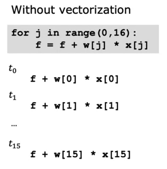
- 직렬적으로 처리
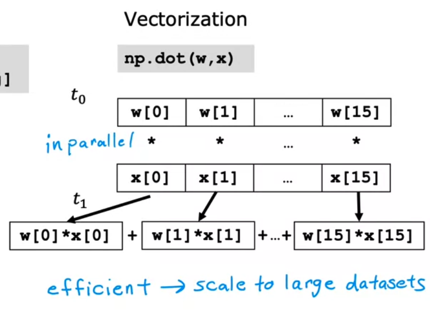
- 병렬적으로 처리
- 벡터화 처리된 코드가 훨씬 빠르고 대규모 데이터 세트에서 알고리즘을 실행하거나 학습시킬 때 효율적이다.
- Gradient Descent 예시
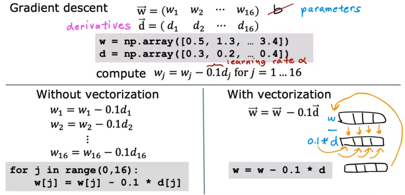
- Vectorization 을 사용하면 선형 회귀를 훨씬 더 효율적으로 구현할 수 있다.
Python Numpy 실습
- Numpy 의 기본 데이터 구조는 동일한 유형 (
dtype)의 요소를 포함하는 인덱싱 가능한 n-dimensional array이다. 여기서 ‘dimension’이라는 용어가 오버로드 되었음을 알 수 있다. 여기서 벡터는 1차원 배열이다. (n,) 을 의미.
Vector Creation
벡터 생성 방법
선형 회귀를 확장하여 여러개의 input feature 를 처리하는 방법을 알아보자. 또한 벡터화 vectorization, 특징 스케일링 feature scaling, 특징 엔지니어링 feature engineering, 다항식 회귀 polynomial regression 등 모델의 훈련과 성능을 개선하기 위한 방법들이 존재한다.
1
2
3
4
# NumPy routines which allocate memory and fill arrays with value
a = np.zeros(4);                print(f"np.zeros(4) :   a = {a}, a shape = {a.shape}, a data type = {a.dtype}")
a = np.zeros((4,));             print(f"np.zeros(4,) :  a = {a}, a shape = {a.shape}, a data type = {a.dtype}")
a = np.random.random_sample(4); print(f"np.random.random_sample(4): a = {a}, a shape = {a.shape}, a data type = {a.dtype}")
1
2
3
np.zeros(4) :   a = [0. 0. 0. 0.], a shape = (4,), a data type = float64
np.zeros(4,) :  a = [0. 0. 0. 0.], a shape = (4,), a data type = float64
np.random.random_sample(4): a = [0.26311627 0.31122847 0.66214921 0.61216887], a shape = (4,), a data type = float64
1
2
3
# NumPy routines which allocate memory and fill arrays with value but do not accept shape as input argument
a = np.arange(4.);              print(f"np.arange(4.):     a = {a}, a shape = {a.shape}, a data type = {a.dtype}")
a = np.random.rand(4);          print(f"np.random.rand(4): a = {a}, a shape = {a.shape}, a data type = {a.dtype}")
1
2
np.arange(4.):     a = [0. 1. 2. 3.], a shape = (4,), a data type = float64
np.random.rand(4): a = [0.09201856 0.10623165 0.29108983 0.30078057], a shape = (4,), a data type = float64
1
2
3
# NumPy routines which allocate memory and fill with user specified values
a = np.array([5,4,3,2]);  print(f"np.array([5,4,3,2]):  a = {a},     a shape = {a.shape}, a data type = {a.dtype}")
a = np.array([5.,4,3,2]); print(f"np.array([5.,4,3,2]): a = {a}, a shape = {a.shape}, a data type = {a.dtype}")
1
2
np.array([5,4,3,2]):  a = [5 4 3 2],     a shape = (4,), a data type = int64
np.array([5.,4,3,2]): a = [5. 4. 3. 2.], a shape = (4,), a data type = float64
Operations on Vectors - 벡터 연산
- Indexing
- 배열 내의 위치에 따라 배열의 요소를 참조하는 것을 의미한다.
1
2
3
4
5
6
7
8
9
10
11
12
13
14
15
16
#vector indexing operations on 1-D vectors
a = np.arange(10)
print(a)

#access an element
print(f"a[2].shape: {a[2].shape} a[2]  = {a[2]}, Accessing an element returns a scalar")

# access the last element, negative indexes count from the end
print(f"a[-1] = {a[-1]}")

#indexs must be within the range of the vector or they will produce and error
try:
    c = a[10]
except Exception as e:
    print("The error message you'll see is:")
    print(e)
1
2
3
4
5
[0 1 2 3 4 5 6 7 8 9]
a[2].shape: () a[2]  = 2, Accessing an element returns a scalar
a[-1] = 9
The error message you'll see is:
index 10 is out of bounds for axis 0 with size 10
- Slicing
- 인덱스를 기반으로 배열에서 요소의 하위 집합을 얻는 것을 의미한다.
1
2
3
4
5
6
7
8
9
10
11
12
13
14
15
16
17
18
#vector slicing operations
a = np.arange(10)
print(f"a         = {a}")

#access 5 consecutive elements (start:stop:step)
c = a[2:7:1];     print("a[2:7:1] = ", c)

# access 3 elements separated by two
c = a[2:7:2];     print("a[2:7:2] = ", c)

# access all elements index 3 and above
c = a[3:];        print("a[3:]    = ", c)

# access all elements below index 3
c = a[:3];        print("a[:3]    = ", c)

# access all elements
c = a[:];         print("a[:]     = ", c)
1
2
3
4
5
6
a         = [0 1 2 3 4 5 6 7 8 9]
a[2:7:1] =  [2 3 4 5 6]
a[2:7:2] =  [2 4 6]
a[3:]    =  [3 4 5 6 7 8 9]
a[:3]    =  [0 1 2]
a[:]     =  [0 1 2 3 4 5 6 7 8 9]
- Vector Operations
1
2
3
4
5
6
7
8
9
10
11
12
13
14
15
16
17
18
19
20
21
22
23
24
25
26
27
28
29
30
31
32
33
34
a = np.array([1,2,3,4])
print(f"a             : {a}")
# negate elements of a
b = -a
print(f"b = -a        : {b}")

# sum all elements of a, returns a scalar
b = np.sum(a)
print(f"b = np.sum(a) : {b}")

b = np.mean(a)
print(f"b = np.mean(a): {b}")

b = a**2
print(f"b = a**2      : {b}")

a = np.array([ 1, 2, 3, 4])
b = np.array([-1,-2, 3, 4])
print(f"Binary operators work element wise: {a + b}")

#try a mismatched vector operation
c = np.array([1, 2])
try:
    d = a + c
except Exception as e:
    print("The error message you'll see is:")
    print(e)


a = np.array([1, 2, 3, 4])

# multiply a by a scalar
b = 5 * a
print(f"b = 5 * a : {b}")
1
2
3
4
5
6
7
8
9
10
11
12
13
a             : [1 2 3 4]
b = -a        : [-1 -2 -3 -4]
b = np.sum(a) : 10
b = np.mean(a): 2.5
b = a**2      : [ 1  4  9 16]

Binary operators work element wise: [0 0 6 8]


The error message you'll see is:
operands could not be broadcast together with shapes (4,) (2,)

b = 5 * a : [ 5 10 15 20]
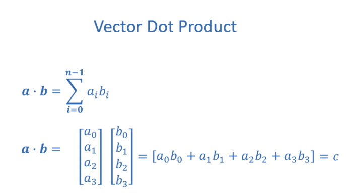
Vector Dot Product - 벡터의 내적
- 내적은 두 벡터의 값을 요소별로 곱한다음 합산하는 과정이다. 두 벡터는 같은 차원이어야함.
1
2
3
4
5
6
7
8
9
10
11
12
13
14
15
16
17
18
19
20
def my_dot(a,b):
    """
   Compute the dot product of two vectors

    Args:
      a (ndarray (n,)):  input vector
      b (ndarray (n,)):  input vector with same dimension as a

    Returns:
      x (scalar):
    """
    x = 0
    for i in range(a.shape[0]):
        x = x + a[i] * b[i]
    return x

# test 1-D
a = np.array([1,2,3,4])
b = np.array([-1,4,3,2])
print(f"my_dot(a, b) = {my_dot(a,b)}")
1
my_dot(a, b) = 24
- Numpy 의 np.dot
1
2
3
4
5
6
7
# test 1-D
a = np.array([1, 2, 3, 4])
b = np.array([-1, 4, 3, 2])
c = np.dot(a, b)
print(f"NumPy 1-D np.dot(a, b) = {c}, np.dot(a, b).shape = {c.shape} ")
c = np.dot(b, a)
print(f"NumPy 1-D np.dot(b, a) = {c}, np.dot(a, b).shape = {c.shape} ")
1
2
NumPy 1-D np.dot(a, b) = 24, np.dot(a, b).shape = ()
NumPy 1-D np.dot(b, a) = 24, np.dot(a, b).shape = ()
- vector vs for loop 속도 비교
1
2
3
4
5
6
7
8
9
10
11
12
13
14
15
16
17
18
19
np.random.seed(1)
a = np.random.rand(10000000)  # very large arrays
b = np.random.rand(10000000)

tic = time.time()  # capture start time
c = np.dot(a, b)
toc = time.time()  # capture end time

print(f"np.dot(a, b) =  {c:.4f}")
print(f"Vectorized version duration: {1000*(toc-tic):.4f} ms ")

tic = time.time()  # capture start time
c = my_dot(a,b)
toc = time.time()  # capture end time

print(f"my_dot(a, b) =  {c:.4f}")
print(f"loop version duration: {1000*(toc-tic):.4f} ms ")

del(a);del(b)  #remove these big arrays from memory
1
2
3
4
5
# mac m2 pro
np.dot(a, b) =  2501072.5817
Vectorized version duration: 15.5680 ms
my_dot(a, b) =  2501072.5817
loop version duration: 1428.7817 ms
Matrix Creation
1
2
3
4
5
6
7
8
a = np.zeros((1, 5))
print(f"a shape = {a.shape}, a = {a}")

a = np.zeros((2, 2))
print(f"a shape = {a.shape}, a = \n {a}")

a = np.random.random_sample((1, 1))
print(f"a shape = {a.shape}, a = {a}")
1
2
3
4
5
a shape = (1, 5), a = [[0. 0. 0. 0. 0.]]
a shape = (2, 2), a =
 [[0. 0.]
 [0. 0.]]
a shape = (1, 1), a = [[0.25371341]]
1
2
3
4
5
6
# NumPy routines which allocate memory and fill with user specified values
a = np.array([[5], [4], [3]]);   print(f" a shape = {a.shape}, np.array: a = \n {a}")
a = np.array([[5],   # One can also
              [4],   # separate values
              [3]]); #into separate rows
print(f" a shape = {a.shape}, np.array: a = \n {a}")
1
2
3
4
5
6
7
8
 a shape = (3, 1), np.array: a =
 [[5]
 [4]
 [3]]
 a shape = (3, 1), np.array: a =
 [[5]
 [4]
 [3]]
- Indexing
1
2
3
4
5
6
7
8
9
#vector indexing operations on matrices
a = np.arange(6).reshape(-1, 2)   #reshape is a convenient way to create matrices
print(f"a.shape: {a.shape}, \na= \n {a}")

#access an element
print(f"\na[2,0].shape:   {a[2, 0].shape}, a[2,0] = {a[2, 0]},     type(a[2,0]) = {type(a[2, 0])} Accessing an element returns a scalar\n")

#access a row
print(f"a[2].shape:   {a[2].shape}, a[2]   = {a[2]}, type(a[2])   = {type(a[2])}")
1
2
3
4
5
6
7
8
9
a.shape: (3, 2),
a=
 [[0 1]
 [2 3]
 [4 5]]

a[2,0].shape:   (), a[2,0] = 4,     type(a[2,0]) = <class 'numpy.int64'> Accessing an element returns a scalar

a[2].shape:   (2,), a[2]   = [4 5], type(a[2])   = <class 'numpy.ndarray'>
- Slicing
1
2
3
4
5
6
7
8
9
10
11
12
13
14
15
16
17
18
#vector 2-D slicing operations
a = np.arange(20).reshape(-1, 10)
print(f"a = \n{a}")

#access 5 consecutive elements (start:stop:step)
print("a[0, 2:7:1] = ", a[0, 2:7:1], ",  a[0, 2:7:1].shape =", a[0, 2:7:1].shape, "a 1-D array")

#access 5 consecutive elements (start:stop:step) in two rows
print("a[:, 2:7:1] = \n", a[:, 2:7:1], ",  a[:, 2:7:1].shape =", a[:, 2:7:1].shape, "a 2-D array")

# access all elements
print("a[:,:] = \n", a[:,:], ",  a[:,:].shape =", a[:,:].shape)

# access all elements in one row (very common usage)
print("a[1,:] = ", a[1,:], ",  a[1,:].shape =", a[1,:].shape, "a 1-D array")
# same as
print("a[1]   = ", a[1],   ",  a[1].shape   =", a[1].shape, "a 1-D array")
1
2
3
4
5
6
7
8
9
10
11
12
a =
[[ 0  1  2  3  4  5  6  7  8  9]
 [10 11 12 13 14 15 16 17 18 19]]
a[0, 2:7:1] =  [2 3 4 5 6] ,  a[0, 2:7:1].shape = (5,) a 1-D array
a[:, 2:7:1] =
 [[ 2  3  4  5  6]
 [12 13 14 15 16]] ,  a[:, 2:7:1].shape = (2, 5) a 2-D array
a[:,:] =
 [[ 0  1  2  3  4  5  6  7  8  9]
 [10 11 12 13 14 15 16 17 18 19]] ,  a[:,:].shape = (2, 10)
a[1,:] =  [10 11 12 13 14 15 16 17 18 19] ,  a[1,:].shape = (10,) a 1-D array
a[1]   =  [10 11 12 13 14 15 16 17 18 19] ,  a[1].shape   = (10,) a 1-D array
다중 선형 회귀를 위한 경사 하강법
- 기존 단일 변수 선형회귀에서는 단 한개의 feature 가지고 진행했었다.
- 다중 선형 회귀는 집의 크기 뿐만아니라, 방의 수 층수 집의 연차 등을 통해 가격을 예측하는데 더 많은 정보를 얻을 수 있다.
- feature 가 2개 이상인 경우
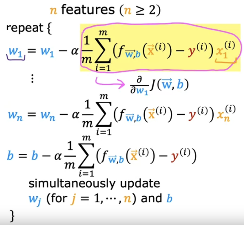
- $w_1, \dots , w_n, b$ 까지 업데이트를 진행한다.
Normal equation - 정규 방정식
- $w, b$ 를 찾기 위한 또 다른 방법으로는 정규 방정식이 존재한다.
- 경사 하강법은 비용함수 $J$ 를 최소화하여 $w, b$ 를 찾는 매우 훌룡한 방법이지만, $w, b$ 를 찾는 또 다른 알고리즘이 존재하는데 이를 정규 방정식이라고 한다.
- 정규 방정식은 오로지 선형 회귀에만 적용된다. 로지스틱 회귀 같은 곳에서는 적용할 수 없음.
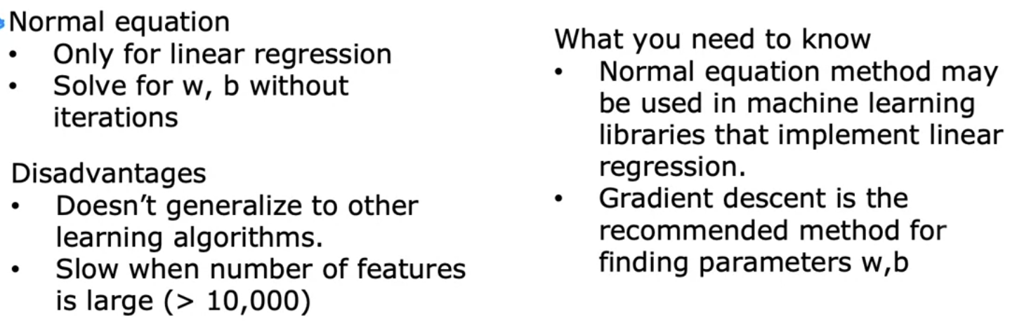
- 장점
- 반복없이 한 번에 $w, b$ 를 해결할 수 있다.
- 단점
- 다른 학습 알고리즘 (로지스틱 회귀, 신경망 등) 에서 일반화되지 않는다.
- feature 의 수가 많으면 정규 방정식은 매우 느리다.
- 주로 어디서 사용하느냐?
- 일부 머신러닝 라이브러리에서는 백엔드 단에서 정규 방정식을 활용하여 $w, b$ 를 구하기도 한다. 경사하강법이 훨씬 낫다.
이 기사는 저작권자의 CC BY 4.0 라이센스를 따릅니다.