Linear Algebra - 1.5 Solution Sets of Linear Algebra

용어 정리

• homogeneous system (제차 선형계)
• nonhomogeneous system (비제차 선형계)
• tirivial solution (자명해)
• nontrivial solution (비자명해)
• particular solution (특수해)
• homogeneous solution (제차해)

Homogeneous Linear Systems - 제차 선형계

• $ A\mathsf{x} = 0 $ 인 matrix equation을 homogeneous linear system 이라고 한다.

• homogeneous linear system 의 특징

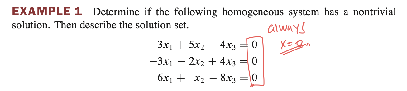
The homogeneous equation $ A\mathsf{x} = 0 $ has a nontrivial solution if and only if the equation has at least one free varialbe.

(1)  항상 최소 하나의 trivial solution을 갖고 있다.
trivial solution은 $ x = 0 $ 을 의미한다.

(2)  nontrivial solution 을 갖는 조건
방정식이 1개 이상의 free variable 을 갖고있으면 nontrivial solution이다.
nontrivial solution은 $ x \ne 0 $ 을 의미한다.
theorem 2 에 따르면, free varialbe 이 없으면 unique solution을 갖고, free variable 이 있으면 infinitely many solution을 갖는다.

nontrivial solution 있는지 확인하기

• homogeneous system 임을 가정하고 풀이를 하기 때문에 항상 우측항은 0이 온다. $ A\mathsf{x} = 0 $ 이므로..

• $A\mathsf{x} = 0$을 augmented matrix로 표현 하고 row reduction을 통해 reduced echelon matrix를 만들어서 free variable이 존재하는지 확인하면 된다.

  

• 3row 가 전부 0 이므로 $ x_3 $는 free varialbe 이다. $ x_1 $은 basic solution, $ x_2 $는 trivial solution.

  

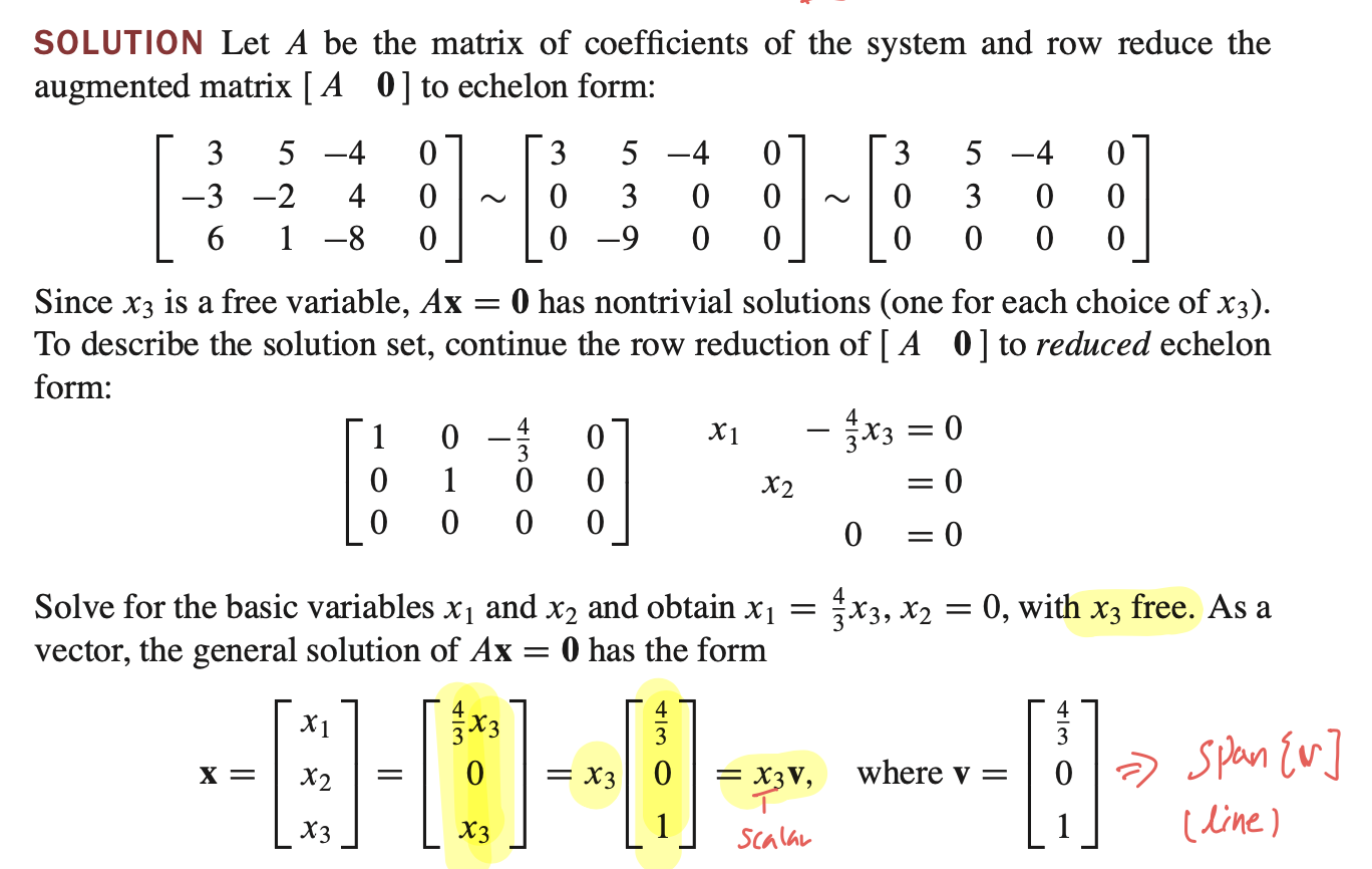
• 이는 $ x_1, x_2, x_3 $ 를 $ x_3 $ 하나로 표현할 수 있기 때문에 벡터의 linear combination으로 표현할 수 있다.

• 따라서 Span{$ v $} 를 의미하며 $ \mathbb{R}^{3} $ 공간에서 직선으로 표현된다.

  

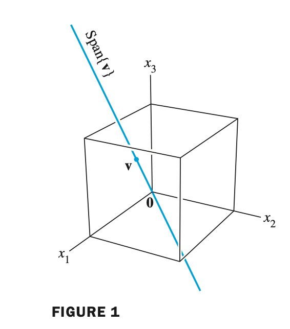
• Span{$ v $}로 표시할수 있다는 의미는 nontrivial solution이 존재한다는 것을 의미한다.
• 왜냐하면 trivial solution은 $ \mathsf{x} = 0 $ 을 의미하므로 x에 해당되는 v가 사라지기 때문..
• And also trivial solution can express as Span{$ 0 $}
• trivial solution은 Span{$0$}로 표현이 가능하다.

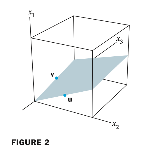
선형 방정식이 하나일때 nontrivial solution 확인하기

• 식이 하나여도 linear system이라고 부를 수 있다.

• $ x_1 $ 을 pivot position 으로 설정하고 풀면 된다.

  

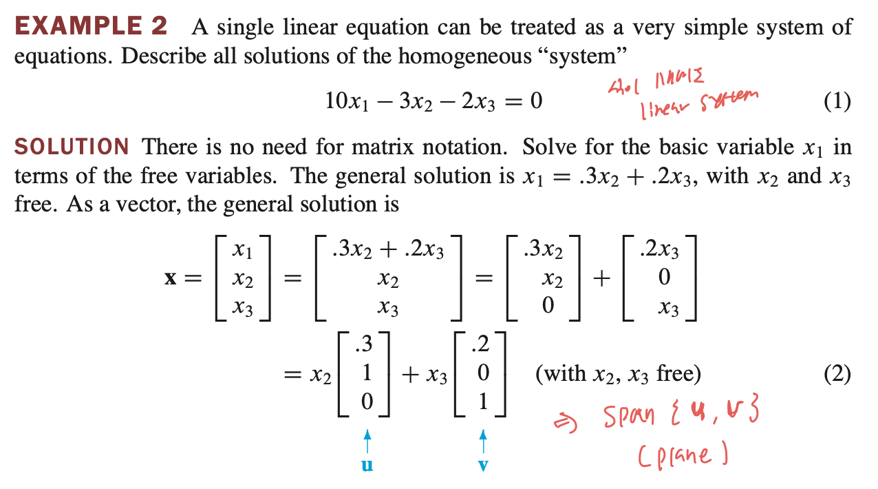
  • $ x_1 $ 은 basic solution, $ x_2, x_3 $ 는 free varialbe이다.
  • 따라서 nontrivial 이 존재하고 두 개의 벡터의 linear combination 으로 표현할 수 있으므로 Span{$ u, v $} 가 된다.

  • $ \mathbb{R}^{3} $ 공간에서 평면으로 표현된다.

    

정리하자면

• Ax = 0 homogeneous linear system 에서 solution set 은 Span{$ v_1, \dots , v_p $} 로 표현할 수 있다.
• 만약 trivial solution이 존재하면 Span{0} 으로 표한한다. (n 공간에서 하나의 점 이므로)
• trivial solution 은 x = 0 이므로 Span{}에서 x = 0 에 해당되는 v는 의미가 없어지게 된다.

• 따라서 nontrivial solution이 없다면 Span{$ v_1, \dots , v_p $} 로 표현할 수 없다.

  
  
  

Nonhomogeneous linear systems - 비제차 선형계

• nonhomogeneous linear system 은 $A\mathsf{x} = b$를 의미한다.

• b 는 nonzero vector 를 의미하며 이는 b의 entry 중 적어도 하나 이상의 entry가 nonzero 임을 의미한다.

  

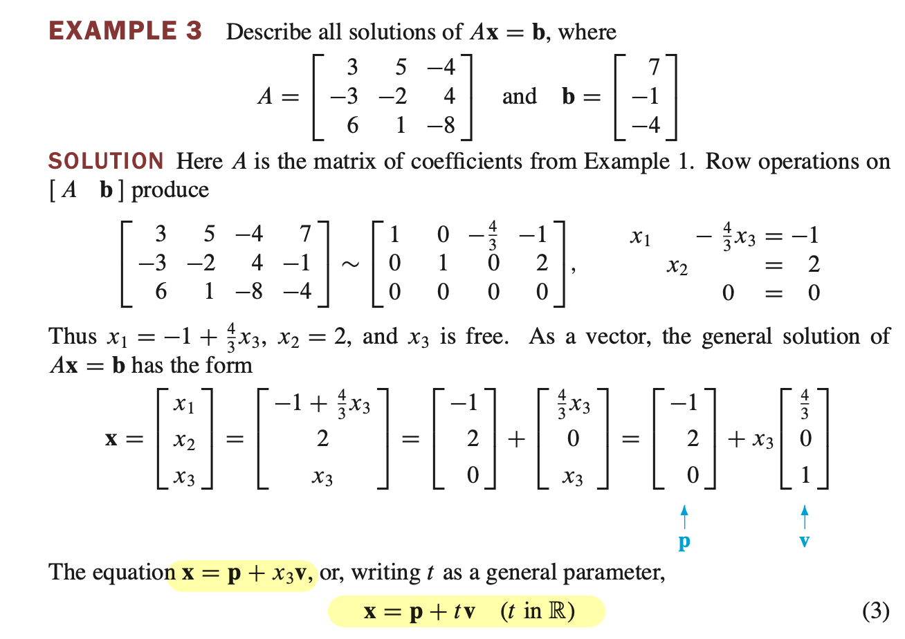
• $x_1$은 basic variable, $x_2$는 nontrivial solution, $x_3$는 free varialbe이다.
• p 를 particular solution, v 를 homogeneous solution 이라고 한다.
• nonhomogeneous linear system 의 solution 은 p (particular solution) 와 v (homogeneous solution)의 합으로 표현된다.
• 이처럼 homogeneous linear system 과 nonhomogeneous linear system은 밀접한 관계를 갖고있다.

Theorem6. Solution Set of Nonhomogeneous Equation
Suppose the equation $ \mathbf{A}\mathsf{x} = \mathbf{b} $ is consistent for some given $ \mathbf{b} $, and let $ \mathbf{p} $ be a solution.
Then the solution set of $ \mathbf{A}\mathsf{x} = \mathbf{b} $ is the set of all vectors of the form $ \mathbf{w} = \mathbf{p} + \mathbf{v}_h $,
where $ \mathbf{v}_h $ is any solution of the homogeneous equation $ A\mathsf{x} = 0 $

nonhomogeneous equation 의 solution set 은 $ \mathbf{w} = \mathbf{p} + \mathbf{v}_h $ 로 표현된다.
여기서 $v_h$ 는 homogeneous equation 의 solution 이다.

The relationship of homogeneous solution and nonhomogeneous solution

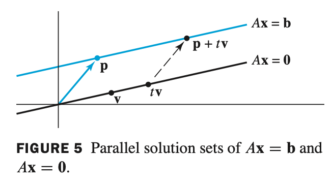
• $ \mathbb{R}^{2} $ 공간

  

• $ \mathbb{R}^{3} $ 공간

  

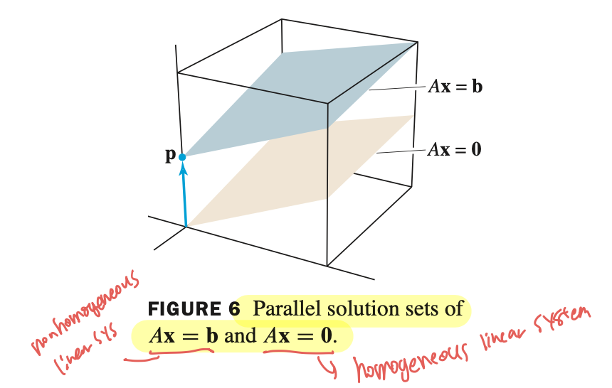
• homogeneous solution 과 nonhomogeneous solution 은 평행 관계를 이룬다.
• $ \mathbf{A}\mathsf{x} = \mathbf{b} $, $ \mathbf{A}\mathsf{x} = 0 $ 의 해는 p (particular solution)에 의해 평행 관계를 이루게 된다.
• 그리고 v (homogeneous solution) 는 평면 공간을 의미한다.