
Linear Algebra - 1.1 Systems of Linear Equations
- Linear Algebra - 1.1 Systems of Linear Equations
- Linear Algebra - 1.2 Row Reduction and Echelon Forms
- Linear Algebra - 1.3 Vector Equations
- Linear Algebra - 1.4 The Matrix Equation Ax=b
- Linear Algebra - 1.5 Solution Sets of Linear Systems
- Linear Algebra - 1.6 Linear Independence and Linear Dependence
- Linear Algebra - 1.7 Introduction to Linear Transformation
- Linear Algebra - 1.8 The Matrix of a Linear Transformation
- Linear Algebra - 2.1 Matrix Operations
- Linear Algebra - 2.2 The Inverse of Matrix
- Linear Algebra - 2.3 Characterizations of Invertible Matrices of
- Linear Algebra - 2.4 Partitioned Matrices
- Linear Algebra - 2.5 Matrix Factorizations, LU Decomposition
- Linear Algebra - 2.6 Subspaces of $\mathbb{R}^n$
- Linear Algebra - 2.7 Dimension and Rank
- Linear Algebra - 3.1 Introduction to Determinants
- Linear Algebra - 3.2 Properties of Determinants
- Linear Algebra - 3.3 Cramer's Rule, Volume, And Linear Transformations
- Linear Algebra - 4.1 Eigenvectors and Eigenvalues
- Linear Algebra - 4.2 The Characteristic Equation
- Linear Algebra - 4.3 Diagonalization
- Linear Algebra - 4.4 Eigenvectors And Linear Transformations
- Linear Algebra - 4.5 Complex Eigenvalues
- Linear Algebra - 5.1 Inner Product And Orthogonality
- Linear Algebra - 5.2 Orthogonal Sets
- Linear Algebra - 5.3 Orthogonal Projections
- Linear Algebra - 5.4 The Gram-Schmidt Process (그람 슈미츠 과정)
- Linear Algebra - 5.5 Least-Square Problems
- Linear Algebra - 6.1 Diagonalization of Symmetric Matrices
- Linear Algebra - 6.2 Quadratic Forms
- Linear Algebra - 6.3 Constrained Optimization
- Linear Algebra - 6.4 SVD, The Singular Value Decomposition
- Linear Algebra - 6.5 Reduced SVD, Pseudoinverse, Matrix Classification, Inverse Algorithm

용어 정리
- linear equation (선형 방정식)
- system of linear equation (선형 방정식 계)
- solution set (해의 집합)
- consistent - exactly one solution, infinitely many solutions
- inconsistent - no solution
- matrix notation (행렬 표기법)
- elimination (소거법)
- row operation (행 연산) - replacement, interchange, scaling
- equivalent (상등)
- row equivalent (행 상등)
선형대수 (Linear Algebra) 는 선형 방정식(Linear Equation)을 풀기 위한 방법론이다.
- 다음과 같은 linear equation 이 있다고 하자, $2x + 3y = 0$
- 여기서 우측의 해 $0$ 을 만족시키는 $x$ 와 $y$ 를 찾아내는 것이다.
- 방정식과 미지수가 하나씩 있으면 solution 을 구하는게 매우 쉽지만
- 방정식 1개에 미지수2개 의 경우 해를 만족시키는 x와 y를 방정식 1개로 찾기는 어렵다.
- 여기서 같은 차원의 방정식이 여러개 있다면? 우리는 두 방정식의 관계를 이용해 해를 찾아낼 수 있다. 이것이 선형대수를 공부하는 목적이다.
선형 방정식 - linear equation
$ x_1,…,x_n$ 변수로 이루어진 선형 방정식은 다음과 같이 쓸 수 있다.
A linear equations in the variables $ x_1, x_2, \dots, x_n $
- 우리는 위와 같은 식을 선형 방정식이라고 부른다.
- 변수 앞에 붙은 $ a_1, a_2, \dots, a_n $ 을 우리는 Coefficients 라고 부른다.
- 여기서 $ a_1, \dots, a_n $ 은 계수(coefficient)이고, $ b $ 는 상수(constant)이다. 이들은 실수(real number) 혹은 복소수(complex number)이다.
- 문제. 그렇다면 다음 두 식은 Linear Equation 인가?
\(4x_1 - 5x_2 = x_1x_2\)
\(x_2 = \sqrt{x_1} - 6\)
정답 : 아니다.
선형 방정식 계 - A system of linear equations (줄여서 linear system)
- a collection of one or more linear equations (같은 변수들을 포함한 선형 방정식이 1개 또는 그 이상의 집합을 의미)
- 선형 방정식이 한 개여도 상관없음
- 선형 방정식의 예시
아래 두 개의 선형 방정식은 선형 방정식 계라고 할 수 있다.
$ x_1 - 2x_2 = -1 $
$ -x_1 + 3x_2 = 3 $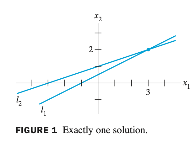
- 위 두 개의 식을 행렬로 표시하면 다음과 같다.
$ \begin{bmatrix} 1 & -2 \\ -1 & 3 \end{bmatrix} \begin{bmatrix} x \\ y \end{bmatrix} = \begin{bmatrix} -1 \\ 3 \end{bmatrix} $
$ A\mathbf{x} = \mathbf{b} $
- 왼쪽부터 순서대로, Coefficient Matrix - 계수행렬(A), unknown vector - 미지수 벡터(x), 우변 벡터(b) 이다.
- Row Picture
- Row picture 란 Row 방향의 방정식을 하나씩 보는 것이다. 예를 들어, 위 식에서 $ x_1 - 2x_2 = -1 $ 의 하나의 방정식을 놓고 봤을 때, 이 방정식이 공간상에서 어떻게 표현되는지, 무엇을 의미하는지를 아는 것이다.
- 선형대수에서 이러한 row 방향의 하나의 방정식은 좌표 공간상에서 직선으로 표현된다. 위 방정식들을 $y=x$ 꼴로 정리해서 풀어보면
$ x_2 = {1 \over 2}x_1 + {1 \over 2} $
$ x_2 = {1 \over 3}x_1 + 1 $
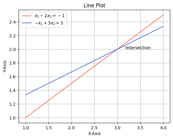
matplotlib 로 작성했다.
- 해당 그래프를 보면 (3,2)에서 교점이 존재하는데, 이것이 linear system 의 해이다.
matplotlib로 작성한 코드
1
2
3
4
5
6
7
8
9
10
11
12
13
14
15
16
17
18
19

import numpy as np
import matplotlib.pyplot as plt

x1 = np.array(range(1, 6)) # system value 의 범위를 의미
x2 = np.array(range(1, 6))
x3 = np.array(range(1, 6))

plt.plot(x1, 1/2 * x1 + 1/2, color='tomato', label="$x_1 - 2x_2 = -1$") # y = x 꼴로 간단히 표현가능
plt.plot(x2, 1/3 * x2 + 1, color='royalblue', label="$-x_1 + 3x_2 = 3$")
plt.xlabel("X-Axis")
plt.ylabel("Y-Axis")
plt.legend()
plt.title('Line Plot')
plt.grid(True)

plt.text(3, 2, "      Intersection")

plt.show()
- Column Picture
$ x_1 \begin{bmatrix} 1 \\ -1 \end{bmatrix} + x_2 \begin{bmatrix} -2 \\ 3 \end{bmatrix} = \begin{bmatrix} -1 \\ 3 \end{bmatrix} $ - 위 방정식을 column 식으로 표현
$ x_1\mathbf{a_1} + x_2\mathbf{a_2} = \mathbf{b} $ - 일반화 한 것
- 우리는 위와 같은 형태를 linear combination (선형 결합)이라고 부르며, 이러한 형태의 연산은 선형대수에서 가장 근본적이며 핵심적인 연산이다.
여기서 $ x_1, x_2, \dots, x_n $ 은 스칼라(가중치)이고, $ \mathbf{a_1}, \mathbf{a_2}, \dots, \mathbf{a_n} $ 은 열 벡터(column vector)이다.

matplotlib로 작성한 코드
1
2
3
4
5
6
7
8
9
10
11
12
13
14
15
16
17
18
19
20
21
22

import numpy as np
import matplotlib.pyplot as plt

x = np.array([1, -1]) # 벡터로도 array 표현이 가능
y = np.array([-2, 3])
lc = 3*x + 2*y # 선형 결합

plt.clf()

plt.arrow(0, 0, x[0], x[1], head_width=0.1, head_length=0.2, color="red", label="$x_1 = [1, -1]$") # 벡터는 arrow 로 표현
plt.arrow(0, 0, y[0], y[1], head_width=0.1, head_length=0.2, color="blue", label="$x_2 = [-2, 3]$")
plt.arrow(0, 0, lc[0], lc[1], head_width=0.1, head_length=0.2, color="green", label="$b = [-1,3]$")

plt.xlabel("$x_1$-axis")
plt.ylabel("$x_2$-axis")

plt.legend()
plt.grid(True)
plt.title('Line Plot')
plt.show()
- 결국 Row Picture 든 Column Picture 든 똑같은 시스템 A를 보는 것이므로 해는 같다.
- 문제를 직선이나 평면 방정식으로 볼것인지, 벡터들의 선형결합으로 볼것인지의 차이일 뿐이다.
해의 집합 - Solution Set
- The set of all possible solutions of the linear system.
- 선형 시스템에서 모든 가능한 해의 집합을 의미한다.
상등 - equivalent
- Two linear systems are called equivalent if they have the same solution set.
- 두 선형 방정식이 상등(equivalent) 하다라는 뜻은 같은 solution set 을 지녔다는 것을 의미한다.
해가 있다 (consistent), 해가 없다(inconsistent)
해가 없다 - inconsistent
no solution 해가 없는 상태 -> inconsistent
$ x_1 - 2x_2 = -1 $
$ -x_1 + 2x_2 = 3 $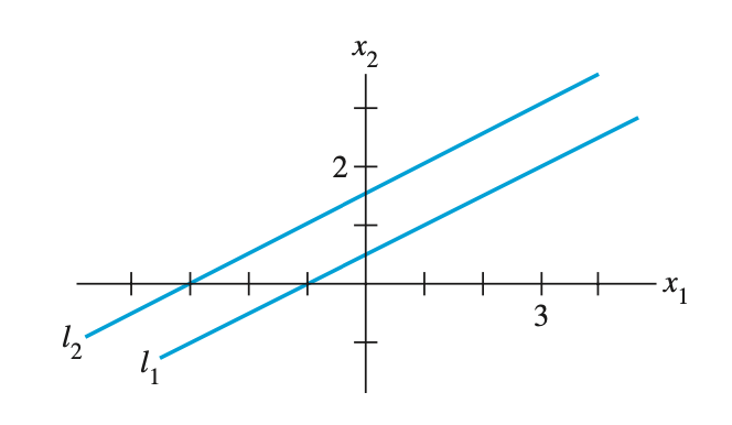
- 이 처럼 두 직선이 평행하게 되면 교차점이 없다. 이 경우에 no solution 이며, 두 방정식은 inconsistent 하다.
해가 있다 - consistent
(i)exactly one solution or (ii)infinitely many solutions 해가 하나이거나 무한히 많을 때 -> consistent
#1. 해가 하나인 경우
$ x_1 - 2x_2 = -1 $ $ -x_1 + 3x_2 = 3 $
#2. 해가 무수히 많은 경우
$ x_1 - 2x_2 = -1 $
$ -x_1 + 2x_2 = 1 $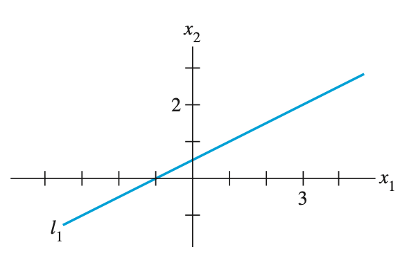
- 정리하자면 선형 방정식 계는 1. no solution, 2. exactly one solution, 3. infinitely many solution 세 가지 경우를 가지고 있다.
- inconsistent 는 no solution, consistent 는 exactly one solution or infinitely many solution을 의미한다.
행렬 표기법 - Matrix notation
- 행렬 표기법은 선형 시스템을 행렬로 표현한 것이다.
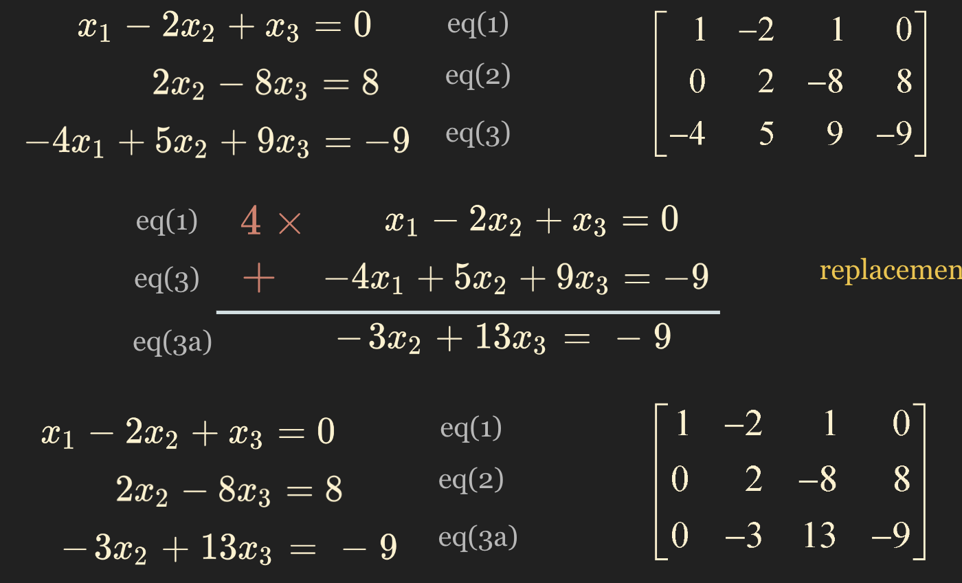
$ x_1 - 2x_2 + x_3 = 0 $
$ 2x_2 - 8x_3 = 8 $
$ -4x_1 + 5x_2 + 9x_3 = -9 $
- 이 3개의 방정식을 행렬로 표기하면 다음과 같다.
(1) 계수 행렬 - coefficient matrix (3x3)
- coefficient matrix 는 b를 제외하고 a만을 행렬로 나타낸 것이다.
$ \begin{bmatrix} \phantom{-}1 & -2 & \phantom{-}1 \\ \phantom{-}0 & \phantom{-}2 & -8 \\ -4 & \phantom{-}5 & \phantom{-}9 \end{bmatrix} $
(2) 첨가 행렬 - augmented matrix (3x4)
- augmented matrix는 b까지 포함한 행렬이다.
$ \begin{bmatrix} \phantom{-}1 & -2 & \phantom{-}1 & \phantom{-}0 \\ \phantom{-}0 & \phantom{-}2 & -8 & \phantom{-}8 \\ -4 & \phantom{-}5 & \phantom{-}9 & -9 \end{bmatrix} $
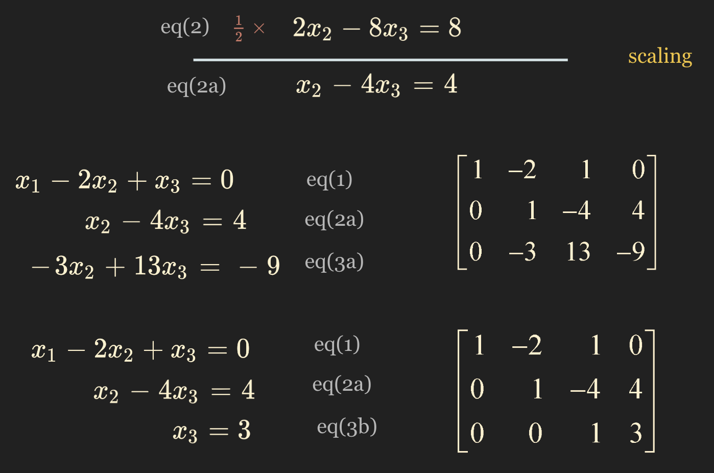
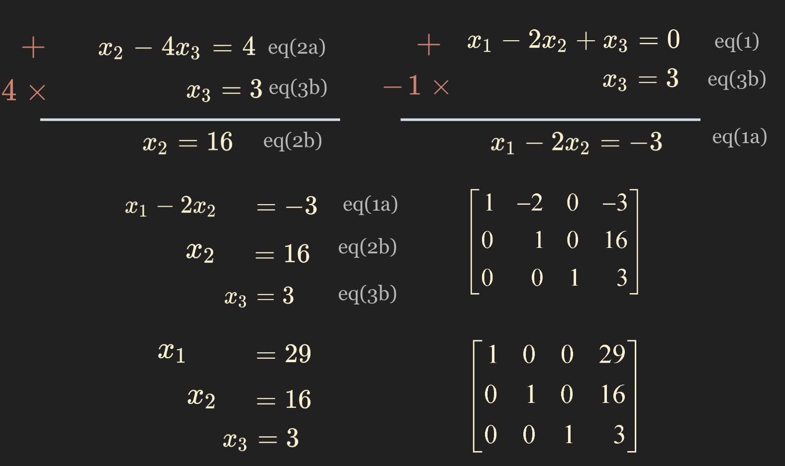
소거법 - elimination
row operation을 통해 elimination을 진행하고 linear equation의 solution을 구할 수 있다.
예제 1. Solve the following system of linear equations
- 우리는 augmented matrix 만을 가지고도 solution을 구할 수 있다.
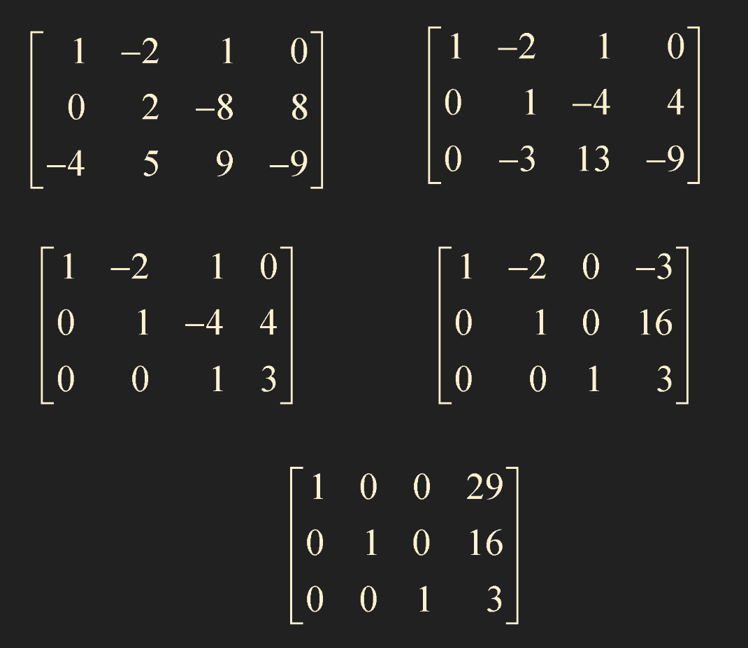
- 우리는 augmented matrix 만을 가지고도 solution을 구할 수 있다.
- $ x_1 = 1, x_2 = 0, x_3 = -1 $ 으로 one solution을 갖고 있으므로 세 방정식은 consistent 하다.
- 또한 같은 solution set을 갖고 있으므로 row equivalent 하다.
- 예제 2. Solve the following system of linear equations
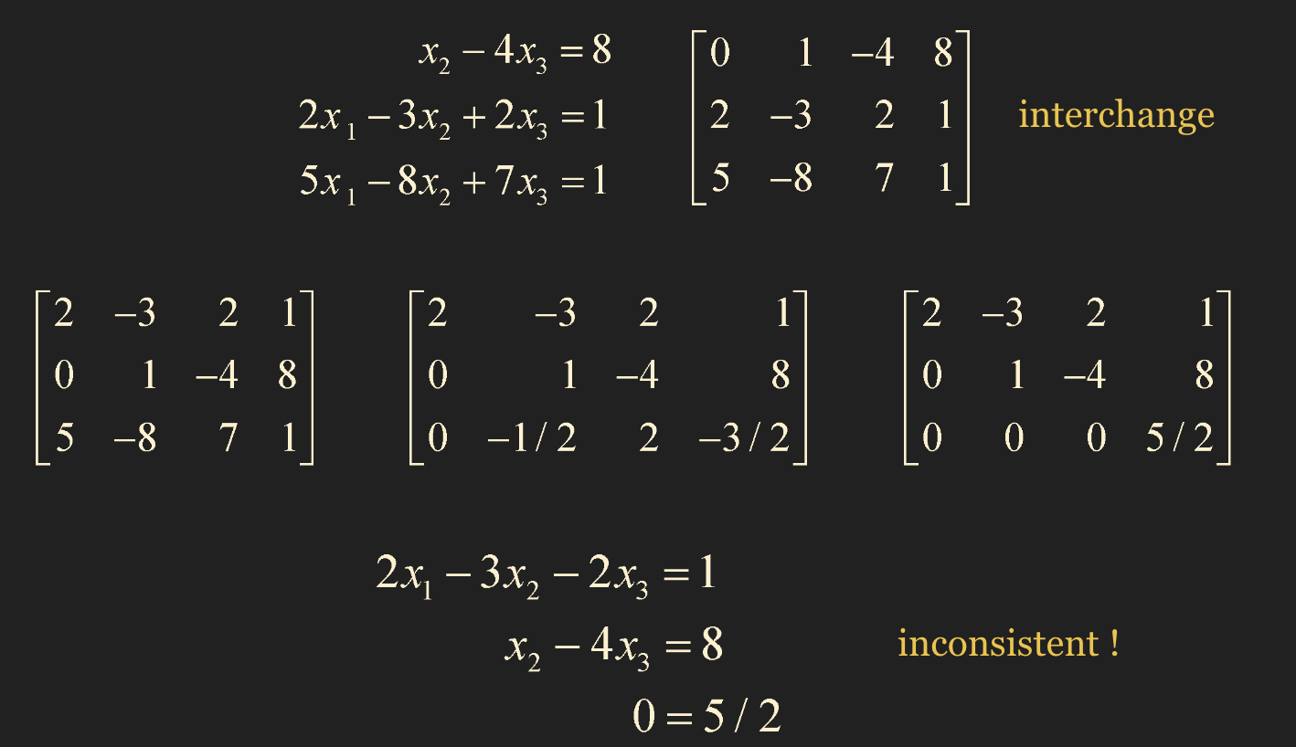
- 행렬에서 좌측 상단을 pivot position 이라고 하는데, 이 pivot position 이 0이 되면 안되므로 interchange 를 실시해야한다.
- row 들 끼리는 자유롭게 interchange 할 수 있다.
- 이 문제는 $ 0 = 5 / 2 $ 이기 때문에 inconsistent 하므로 해가 없다.
행 연산 - Elementary row operations
- replacement
- interchange
- scaling
위 3가지 row operation 을 통해 최종 계산한 결과 값이랑 최초의 행렬이랑 같다. -> row equivalent 하다.
- We say two matrices are row equivalent if there is a sequence of elementary row operations that transforms one matrix into the other.
- If the augmented matrices of two linear systems are row equivalent, then the tow systems have the same solution set. (두 augmented matrices 가 row equivalent 하다라는 말은 같은 solution set을 가지고 있다라는 뜻.)
행 상등 - row equivalent
- row operation을 통해 하나의 matrix 를 다른 matrix로 변환된다면 두 matrix 는 row equivalent 하다고 할 수있다.
- 두 linear system 이 row equivalent 하다면 두 linear system은 have same solution set.