
Linear Algebra - 6.4 SVD, The Singular Value Decomposition

- Linear Algebra - 1.1 Systems of Linear Equations
- Linear Algebra - 1.2 Row Reduction and Echelon Forms
- Linear Algebra - 1.3 Vector Equations
- Linear Algebra - 1.4 The Matrix Equation Ax=b
- Linear Algebra - 1.5 Solution Sets of Linear Systems
- Linear Algebra - 1.6 Linear Independence and Linear Dependence
- Linear Algebra - 1.7 Introduction to Linear Transformation
- Linear Algebra - 1.8 The Matrix of a Linear Transformation
- Linear Algebra - 2.1 Matrix Operations
- Linear Algebra - 2.2 The Inverse of Matrix
- Linear Algebra - 2.3 Characterizations of Invertible Matrices of
- Linear Algebra - 2.4 Partitioned Matrices
- Linear Algebra - 2.5 Matrix Factorizations, LU Decomposition
- Linear Algebra - 2.6 Subspaces of $\mathbb{R}^n$
- Linear Algebra - 2.7 Dimension and Rank
- Linear Algebra - 3.1 Introduction to Determinants
- Linear Algebra - 3.2 Properties of Determinants
- Linear Algebra - 3.3 Cramer's Rule, Volume, And Linear Transformations
- Linear Algebra - 4.1 Eigenvectors and Eigenvalues
- Linear Algebra - 4.2 The Characteristic Equation
- Linear Algebra - 4.3 Diagonalization
- Linear Algebra - 4.4 Eigenvectors And Linear Transformations
- Linear Algebra - 4.5 Complex Eigenvalues
- Linear Algebra - 5.1 Inner Product And Orthogonality
- Linear Algebra - 5.2 Orthogonal Sets
- Linear Algebra - 5.3 Orthogonal Projections
- Linear Algebra - 5.4 The Gram-Schmidt Process (그람 슈미츠 과정)
- Linear Algebra - 5.5 Least-Square Problems
- Linear Algebra - 6.1 Diagonalization of Symmetric Matrices
- Linear Algebra - 6.2 Quadratic Forms
- Linear Algebra - 6.3 Constrained Optimization
- Linear Algebra - 6.4 SVD, The Singular Value Decomposition
- Linear Algebra - 6.5 Reduced SVD, Pseudoinverse, Matrix Classification, Inverse Algorithm

용어 정리
- Singular Value - 특이값
- Singular Value Decomposition - 특이값 분해
SVD, Singular Value Decomposition 란?
- 여태껏 배웠던 모든 것은 다 SVD를 배우기 위해 빌드업을 한 것이다.. 선형대수의 꽃 SVD에 대해 알아보자.
6.1 애서 배운 symmetric matrix 의 diagonalization 은 많은 분야에 적용할 수 있다. 하지만, 모든 행렬이 $A = PDP^{-1}$ 형태로 분해되지 않는다. 특히 $D$ 가 diagonal matrix 이기 때문에 $A$ 는 $m \times m$ matrix 이어야만 diagonalization 이 가능했었다.
- 하지만, SVD(Singular Value Decomposition)는 꼭 square matrix가 아니더라도 $m \times n$ matrix 이여도 diagonalization 이 가능하다고 보면된다.
Singular Values of an $m \times n$ Matrix - $m \times n$ matrix 의 특이값
Let $A$ be an $m \times n$ matrix.
- $A$ 행렬이 $m \times n$ 행렬이라고 가정하자.
$A^TA$ is an $n \times n$ symmetric matrix. $\quad \quad (A^TA)^T = A^TA^{TT} = A^TA$
- $A^TA$ 는 $n \times n$ symmetric matrix 이다.
- symmetric matrix 인지 증명하기 위해서 $A^TA$ 에 transpose 를 해주면 $(A^TA)^T = A^TA^{TT} = A^TA$ symmetric 임을 확인할 수 있다.
$A^TA$ is orthogonally diagonalizable $\quad \quad P = [\mathbf{v}_1 \quad \dots \quad \mathbf{v}_n] $
- 여기서 주의할 점! $A$ 행렬이 symmetric 이 아니라 $A^TA$ 가 symmetric 하므로 $A^TA$ 에 대한 특성을 알아보고 있는것이다.
- $A^TA$ 는 symmetric matrix 이므로 동치관계인 orthogonally diagonalizable 하다.
- orthogonally diagonalize 를 진행하면 $P$ 행렬의 column vector 들은 $ P = [\mathbf{v}_1 \quad \dots \quad \mathbf{v}_n] $ 이 된다.
{$\mathbf{v}_1 , \dots , \mathbf{v}_n$} is orthonormal basis for $\mathbb{R}^n$ , consisting of eigenvalues of $A^TA$
- 따라서 $P$ 행렬의 column vector 들은 $A^TA$ 의 eigenvector 이다.
$\lambda _1, \dots , \lambda _n$ be the associated eigenvalues of $A^TA$
- $A^TA$ 의 eigenvector 가 n 개 있으므로, 그에 대응하는 eigenvalue 도 n개로 대응한다.
$ \lVert A\mathbf{v}_i \rVert^2 = (A\mathbf{v}_i)^T(A\mathbf{v}_i) = \mathbf{v}_i^TA^TA\mathbf{v}_i = \mathbf{v}_i^T\lambda _i\mathbf{v}_i = \lambda _i $ -> nonneagtive!
- 여기서 $\lVert A\mathbf{v}_i \rVert^2$ 즉 $A\mathbf{v}_i$ 의 length 를 알아보자.
- $\lVert A\mathbf{v}_i \rVert^2$ 은 $(A\mathbf{v}_i)^T(A\mathbf{v}_i)$ 으로 내적이 되므로 이를 풀어 써보면
- 여기서 $A^TA\mathbf{v}_i$ 는 $A\mathbf{x} = \lambda \mathbf{x}$ 형식으로 나타낼 수 있으므로 $\lambda _i\mathbf{v}_i$ 로 표현이 가능하다.
- 여기서 eigenvalue $\lambda _i$ 는 scalar 이므로 앞으로 빼고
- $\mathbf{v}_i$ 는 위에서 orthonormal basis 이므로 $\mathbf{v}_i^T\mathbf{v}_i = 1$ 이된다.
$ \lambda _1 \ge\lambda _2 \ge \dots \ge \lambda _n \le 0 $
- length 의 square root 는 항상 $ \lVert A\mathbf{v}_i \rVert^2 \ge 0 $ 이므로.. eigenvalue $\lambda _i$ 는 nonnegative 하다는 성질 또한 확인할 수 있다.
The singular values of $A$ are the square roots of the eigenvalues of $A^TA$
\[\sigma _i = \sqrt{\lambda _i}\]
- 정리하면 singular value 는 $\lVert A\mathbf{v}_i \rVert^2$ 의 length 이다.
- 즉 $A^TA$ 의 eigenvalue 에 square root 를 한 값이 singular value 이다.
- 따라서, singular value 는 nonnegative 하다.
Example 1
Let $A = \begin{bmatrix} 4 & 11 & 14 \\ 8 & 7 & -2 \end{bmatrix} $ , find the singular values of $A$ and find a unit vector $\mathbf{x}$ at which the length $\lVert A\mathbf{x} \rVert$ is maximized.
- $A$ 행렬의 singular value 를 구하기 위해 $A^TA$ 를 구해보면
- characteristic equation 을 풀어 $A^TA$ 의 eigenvalue 들을 구하면
- singular value 를 $A^TA$ 의 eigenvalues 에 square root 를 씌우면 구할 수 있으므로
- 또한 문제에서는 $\lVert A\mathbf{x} \rVert$ 의 length 가 최대가 되는 지점을 구하라고 명시하고 있으므로
- $\lVert A\mathbf{x} \rVert$ 의 length 가 최대가 되는 지점은 $\lVert A\mathbf{x} \rVert^2$ 가 최대가 되는 지점과 같다.
- 위 식을 자세히 보면 quadratic form 이다.
$\lVert \mathbf{x} \rVert = 1$ 제약 조건 하에서의 최대값을 구하면 되는 것이다.
- 6.3 에서 배운대로 제약 조건이 있는 quadratic form 의 최대값은 eigenvalue 의 최대값이므로 $\lambda _1 = 360$ 을 이용해서 unit eigenvector 를 구해보자.
- augmented matrix 로 조합하여 row reduction 을 하면 다음과 같은 eigenvector 가 만들어진다.
추가적으로 $A\mathbf{v}_1,A\mathbf{v}_2,A\mathbf{v}_3$ 는 각각 orthogonal 한 관계에 있다.
- maximum of $\lVert A\mathbf{x} \rVert^2 = 360 $ 이므로 우리가 구해야할 최대값은
maximum of $\lVert A\mathbf{x} \rVert = 6\sqrt{10}$ 이다.
- 정리하자면, $\lVert A\mathbf{x} \rVert$ 의 최대값은 singular value 이다.
Theorem9.
Let {$\mathbf{v}_1 , \dots , \mathbf{v}_n$} is orthonormal basis or $\mathbb{R}^n$ consisting of eigenvectosr of $A^TA$ ,
arranged so that the corresponding eigenvaleus of $A^TA$ satisfy $\lambda _1 \ge \dots \ge \lambda _n$ , and
suppose $A$ has $r$ nonzero singular values.
Then {$A\mathbf{v}_1 , \dots , A\mathbf{v}_r$} is an orthogonal basis for Col $A$ , and rank $A = r$
- $A^TA$ 가 symmetric matrix 이므로 eigenvector 인 $\mathbf{v}$ 는 orhtonormal 벡터이다.
- 따라서 $A\mathbf{v}_1 , \dots , A\mathbf{v}_n$ 은 orthogonal set 인데 여기서 $\lVert A\mathbf{v} \rVert$ 의 length 는 singular value 라고 앞에서 배웠다.
theorem9를 이용하여 SVD 를 증명할 수 있다.
- 증명
- $i \ne j$ 라고 가정하고 다음 두 벡터를 내적하면
- $\mathbf{v}_i^T \cdot \mathbf{v}_j$ 내적은 0이 되기 때문에.. 0 이된다.
- 그러므로 $A\mathbf{v}_1 , \dots , A\mathbf{v}_n$ 은 orthogonal set 이고 $A\mathbf{v}_i \ne 0$ 이면 $i$ 의 인덱스는 다음과 같다. $1 \le i \le r$
그렇다면 $A\mathbf{v}_i = 0$ 이 되는 경우는 $r + 1 \le i \le n$ 이라고 생각할 수 있다. 이말은 $A\mathbf{v}_i$ 의 length 가 0 이며 $\lambda _i$ 또한 0이라는 말이다.
- 따라서 $A\mathbf{v}_1 , \dots , \mathbf{v}_r$ 은 nonzero vector 이고 orthogonal set 이기 때문에, linearly independent set 이라고 볼 수 있다.
- 그리고 여기서 $\mathbf{y} \; \mbox{in} \; \mbox{Col} A$ 즉, 벡터 $\mathbf{y}$ 가 $A$ 의 column space 에 있다고 가정하면 다음과 같이 표현할 수 있다.
- 그리고 $\mathbf{x}$ 벡터가 이미 $\mathbb{R}^n$ space 에 있으므로 다음과 같이 linear combination 형태로 표현가능하다.
- 여기서 우리는 아까 위에서 $A\mathbf{v}_{r+1} \dots A\mathbf{v}_n$ 까지는 0 벡터임을 알고 있으므로
- undetermined 와 overdetermined 에 대해 잠시 살펴보면..
$m < n \quad \mbox{undetermined}$ 이면 $ \mbox{rank} A \le m $ 이고 $ r \le m $ 이다.
$m > n \quad \mbox{overdetermined}$ 이면 $ r \le n < m $ 이다.
- 이말인 즉슨, 어떤 상황이든 $r$ 은 $m$ 이하 이다.
Singular Value Decomposition, SVD - 특이값 분해

- SVD 를 배우기 전 위와 같이 $m \times n$ 행렬 $\Sigma$ 를 정의하자. $\Sigma$ 는 $r$ 개의 singular value 가 diagonal entries 인 $r \times r$ 행렬 $D$ 를 포함하는 block matrix 이다.
- 여기서 $r$ 은 $m, n$ 을 초과하지 않는다.
Theorem10. The Singular Value Decomposition
Let $A$ be an $m \times n$ matrix with rank $r$ . Then there exists an $m \times n$ matrix $\; \Sigma \;$ as in (a) for which the diagonal entries in $D$ are the first $r$ singular values of $A$ , $\; \sigma _1 \ge \sigma _2 \ge \dots \ge \sigma _r > 0 $ ,
and there exists an $m \times m$ orthogonal matrix $U$ and an $n \times n$ orthogonal matrix $V$ such that
\(A = U\Sigma V^T\)
columns of $U$ : left singular vectors of $A$ $\quad \quad$ columns of $V$ : right singular vectors of $A$
- $ A\mathbf{v}_1 , \dots , A\mathbf{v}_r $ 은 nonzero 이며, $\mathbb{R}^m$ space 에 있는 $\mbox{Col} \, A$ 의 orhtogonal basis 이다. 또한 $\mathbf{v}_i$ 는 $\mathbb{R}^n$ space 에 있다.
- 여기서 $ A\mathbf{v}_1 , \dots , A\mathbf{v}_r $ 을 Normalize 하면 $\mathbf{u}_1 , \dots , \mathbf{u}_r$ 이 된다.
- 우리가 배운 Normalize 공식으로 풀어보면 다음과 같다.
- 여기서 $\lVert A\mathbf{v}_i \rVert$ 는 singular value $\sigma _i$ 이므로
- 따라서 singular value 를 이항시키면 다음 식을 구할 수 있다.
$\mathbf{u}_i$ 는 $\mathbb{R}^m$ space 에 존재하고, $r \le m$ 이다.
- linearly independent set 인 $\mathbf{u}_1 , \dots , \mathbf{u}_r$ 을 \(\mathbf{u}_{r+1} , \dots , \mathbf{u}_m\) 까지 추가를 해서 orthonormal basis 를 만들 수 있다.
- 여기서 $m \times m$ 행렬인 $U = [\mathbf{u}_1 \; \mathbf{u}_2 \; \dots \; \mathbf{u}_m]$ 와 $n \times n$ 행렬인 $V = [\mathbf{v}_1 \; \mathbf{v}_2 \; \dots \; \mathbf{v}_n]$ 이 존재한다고 하면
- 여기서 위에서 구한 식 $A\mathbf{v}_i = \sigma _i \mathbf{u}_i$ 를 대입하면
- 그리고 $U\Sigma$ 를 구해보자. $\Sigma$ 행렬은 $r \times r$ 의 diagonal terms 인 $\sigma _1 , \dots , \sigma _r$ 을 지니는 $D$ 행렬과 나머지 $m \times n$ 은 0을 지니는 block matrix 형태이다.
- 두 식이 똑같음을 확인할 수 있으므로 다음과 같이 나타낼 수 있다.
- 또한 $V$ 의 set 은 $n \times n$ 의 square matrix 이며 orthonormal한 관계이므로 $V^{-1} = V^T$ 이다.
- 이 성질을 이용하여 양변에 $V^T$ 를 곱해주면 SVD(Singular Value Decomposition) 이 나온다는 것을 증명할 수 있다.
Example 2
Let $A = \begin{bmatrix} 4 & 11 & 14 \\ 8 & 7 & -2 \end{bmatrix} $ , construct a singular value decomposition of $A$ .
$A$ 행렬이 $2 \times 3$ 이므로, $U : 2 \times 2 , \Sigma : 2 \times 3 , V : 3 \times 3$ 임을 확인하고 진행하자.
- $A^TA$ 는 symmetric matrix 이므로 orthogonally Diagonalize 하다.
- $A^TA$ 의 eigenvalues 를 구하기 위해 다음의 characteristic equation 을 풀면
- $ \lambda _1 = 360 \quad \lambda _2 = 90 \quad \lambda _3 = 0 $ 이고 $\mbox{rank} \; A = 2$ 이다.
- 주의할점은 여기서 이미 rank 가 2 인것을 확인했으므로, 3 번째 singular value 는 무조건 $\sigma _3 = 0$ 이 된다.
- 그리고 바로 $\sigma _i = \sqrt{\lambda _i}$ 식을 이용하여 singular values 를 구할 수 있다.
$ \sigma _1 = 6\sqrt{10} \quad \sigma _2 = 3\sqrt{10} \quad \sigma _3 = 0 $
- orthonormal eigenvectors 을 구하기 위해 다음 행렬 방정식을 풀어야한다.
- 만약 multiplicity 가 2 이상인 중복되는 eigenvalue 가 나오게 된다면, Gram-Schmidt Process 를 사용해서 풀어야한다.
- eigenvector 들을 구하고 Normalize 를 하게 되면 다음과 같다.
$\mathbf{v}_1 = \begin{bmatrix} 1/3 \\ 2/3 \\ 2/3 \end{bmatrix} \quad \mathbf{v}_2 = \begin{bmatrix} -2/3 \\ -1/3 \\ 2/3 \end{bmatrix} \quad \mathbf{v}_3 = \begin{bmatrix} 2/3 \\ -2/3 \\ 1/3 \end{bmatrix}$
- 따라서 orthonormal eigenvectors 로 구성한 $V$ 행렬과 singular values 로 구성한 $\Sigma$ 행렬은 다음과 같다.
- 행렬 $U$ 를 구하기 위해서 $A\mathbf{v}$ 들을 normalize 해주면 되고, $A\mathbf{v}$ 의 length 인 $\lVert A\mathbf{v} \rVert$ 는 singular value $\sigma$ 임을 우리가 알고있으므로
- 여기서 $U$ 행렬은 $2 \times 2$ 이고 $\mathbf{u}_1, \mathbf{u}_2$ 는 서로 orthogonal한 관계에 있으므로 $\mathbf{u}_1, \mathbf{u}_2$ 는 $\mathbb{R}^2$ space 를 span 한다.
- 따라서 $U$ 행렬은 $\mathbf{u}_1, \mathbf{u}_2$ 를 column vector 로 가지게 된다.
- 최종적으로 $A$ 행렬을 SVD 하면 다음과 같다.
Example 3
Let $A = \begin{bmatrix} 1 & -1 \\ -2 & 2 \\ 2 & -2 \end{bmatrix} $ , construct a singular value decomposition of $A$ .
- $A$ 행렬이 $3 \times 2$ 이므로, $U : 3 \times 3 , \Sigma : 3 \times 2 , V : 2 \times 2$ 임을 확인하고 진행하자.
- characteristic equation $ A^TA - \lambda I = 0 $ 을 풀어서 eigenvalues 를 구하면
- $\lambda _1 = 18 \quad \lambda _2 = 0$ 이고 $\mbox{rank} \; A = 1$ 이다.
singular values 를 구해보면 $\sigma _1 = 3\sqrt{2} \quad \sigma _2 = 0$ 이다.
- eigenvectors 를 구하기 위해 $ (A^TA - \lambda I)\mathbf{x} = 0 $ 행렬식을 풀면
- 따라서 $V, \Sigma$ 는 다음과 같다.
- $U$ 를 구하기 위해서 $A\mathbf{v}$ 를 normalize 를 해주면
- 하지만, 여기서 $ \mathbf{u}_2, \mathbf{u}_3 $ 를 알 수 없으므로 찾아야 한다..
- $\mathbb{R}^3$ space 의 orthonormal basis 인 $ \mathbf{u}_1 ,\mathbf{u}_2, \mathbf{u}_3 $ 를 찾아야 한다.
- $ \mathbf{u}_1 ,\mathbf{u}_2, \mathbf{u}_3 $ 가 각각 orthonormal 하므로 다음 처럼 가정할 수 있다.
- $\mathbf{u}_2, \mathbf{u}_3$ 에 대해 $\mathbf{u}_1^T \mathbf{x} = 0$ 을 만족한다.
- $x_2, x_3$ 를 free variable 로 지니는 general solution 으로 표현할 수 있다.
- $\mathbf{w}_2 = \begin{bmatrix} 2 \\ 1 \\ 0 \end{bmatrix} \quad \mathbf{w}_3 = \begin{bmatrix} -2 \\ 0 \\ 1 \end{bmatrix} $ 이고
- 여기서 $\mathbf{u}_1$ 을 기준으로 $\mathbf{w}_2, \mathbf{w}_3$ 를 orthogonal basis 로 만드는 방법인 Gram-Schmidt Process 를 사용하면 된다!
- 하지만, $\mathbf{u}_2, \mathbf{u}_3$ 는 unique 하지않다. 이를 시각적으로 살펴보면
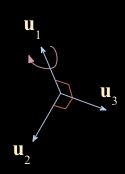
- $\mathbf{u}_1, \mathbf{u}_2, \mathbf{u}_3$ 가 orthonormal 하게 만들었는데, 여기서 $\mathbf{u}_1$ 축을 기준으로 회전을 하게 되면 $ \mathbf{u}_2, \mathbf{u}_3$ 벡터의 방향이 달라지지만 orthonormal basis 를 그대로 유지하게 되므로 사람마다 결과 값의 차이가 존재한다.
- $U = \begin{bmatrix} 1/3 & 2/\sqrt{5} & -2/\sqrt{45} \\ -2/3 & 1/\sqrt{5} & 4/\sqrt{45} \\ 2/3 & 0 & 5/\sqrt{45} \end{bmatrix} $ 이고 최종적으로 SVD 를 구하면
Bases for Fundamental Subspaces
\[A = U\Sigma V^T\]
- $A : m \times n \quad U : m \times m \quad \Sigma : m \times n \quad V : n \times n $ 이고 $\mbox{rank} \; A = r$ 일 때
- 여기서 $U$ vector set 들은 $A$ 의 left singular vectors, $V$ vector set 들은 $A$ 의 right singular vectors 였다.
- 따라서 left singular vectors 인 $\mathbf{u}_1 , \dots, \mathbf{u}_r$ 은 orthogonal basis 인 $A\mathbf{v}_1 , \dots , A\mathbf{v}_r$ 을 Normalize 한 결과이다.
$\mathbf{u}_1 , \dots, \mathbf{u}_r$ set은 Col $A$ 의 orthonormal basis 이다.
- 여기서 주목해야할 점은 Chapter5.1 의 Theorem3 정리인데, 내용은 다음과 같다.
- $A$ 행렬이 $m \times n$ 일 때, \((\mbox{Row}\; A)^{\perp} = \mbox{Nul} \; A \quad \mbox{and} \quad (\mbox{Col} \; A)^{\perp} = \mbox{Nul} \; A^{\perp}\) 이므로
- \(\mathbf{u}_{r+1} , \dots , \mathbf{u}_m\) 은 $\mbox{Nul} \; A^T$ 의 orthonormal basis 이다.
- right singular vectors 인 $\mathbf{v}_1 , \dots , \mathbf{v}_n$ 를 생각해보자
- \(A\mathbf{v}_{r+1} = 0 , \dots , A\mathbf{v}_n = 0\) 이므로 $\mbox{Nul} \; A$ space 에 존재한다.
- $\mbox{rank} \; A = r$ 이면 $\mbox{dim} \; \mbox{Nul} \; A = n - r$ 이므로
- \(\mathbf{v}_{r+1}, \dots , \mathbf{v}_n\) 은 $\mbox{Nul} \; A$ space 의 orthonormal basis 들이고 위의 theorem 3 에 따라서
- $\mathbf{v}_1 , \dots , \mathbf{v}_r$ 은 $\mbox{Row} \; A$ space 의 orthonormal basis 가 성립한다.
- 위 내용을 그림으로 표현하면 다음과 같다.
- \((\mbox{Row}\; A)^{\perp} = \mbox{Nul} \; A \quad \mbox{and} \quad (\mbox{Col} \; A)^{\perp} = \mbox{Nul} \; A^{\perp}\) 이 내용을 숙지하고 그림을 보면
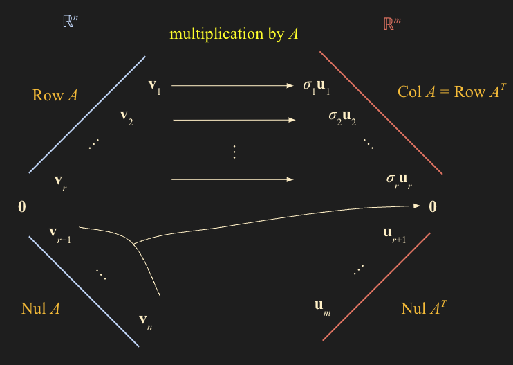
- $\mbox{Row}\; A$ 의 perpendicular 는 $\mbox{Nul}\; A$ 이고 여기에 $A$ 를 multiplication 해주면
- 우리가 SVD를 하면서 배웠던 $A\mathbf{v}_1 = \sigma _1\mathbf{u}_1 , \dots , A\mathbf{v}_r = \sigma _r \mathbf{u}_r$ 가 되고
- Null space 의 vector 들은 $A\mathbf{v}_{r+1} = 0 , \dots , A\mathbf{v}_n = 0$ 전부 제로 벡터로 간다.
\[\mathbf{v}_1 = \begin{bmatrix} 1/\sqrt{2} \\\ -1/\sqrt{2} \end{bmatrix} \quad \mathbf{v}_2 = \begin{bmatrix} 1/\sqrt{2} \\\ 1/\sqrt{2} \end{bmatrix}\] \[\sigma _1 = 3\sqrt{2} \quad \sigma _2 = 0 \quad \quad \mbox{rank} \; A = 1\]Example 3
Let $A = \begin{bmatrix} 1 & -1 \\ -2 & 2 \\ 2 & -2 \end{bmatrix} $ 일때 SVD 를 기하학적으로 살펴보자.
- Gram Schmidt Process
- 여기서 $\mathbf{v}_1, \mathbf{v}_2$ 는 $\mathbb{R}^2$ space 에 존재하고, 반지름이 1인 unit vector 이므로 다음 그림처럼 반드시 원 안에 존재한다.
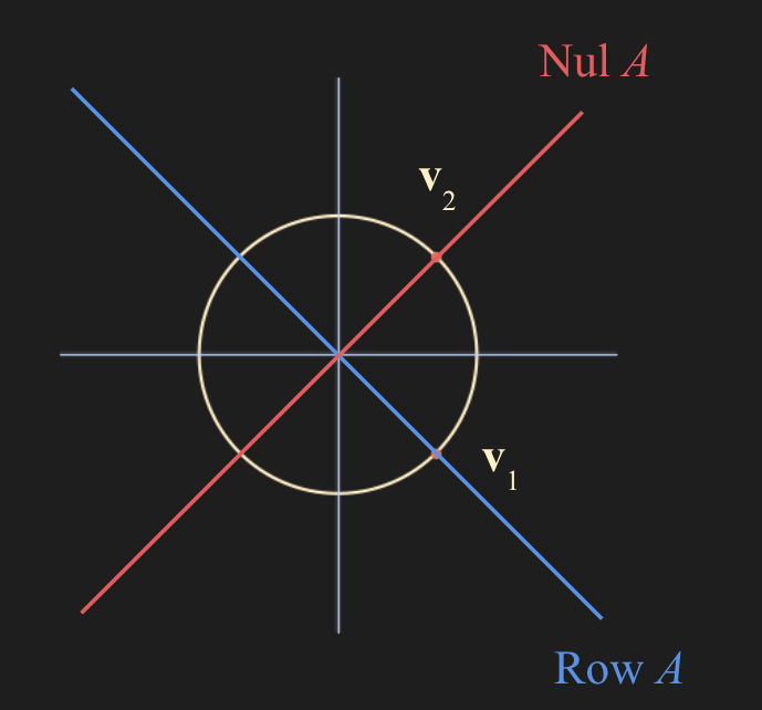
$\mathbf{v}_1$ 의 Span은 $\mbox{Row} \; A$ space에 존재하고 $\mbox{Row} \; A$ 의 perpendicular 는 바로 $\mbox{Nul} \; A$ space, 즉 $\mathbf{v}_2$ 의 span 이다.
그리고 여기서 $A$ multiplication 을 해주면 다음과 같다.
- $\mathbf{v}_2$ 는 Nul Space 에 있기 때문에 당연히 0 벡터로 간다.
- $A\mathbf{v}_1$ 은 $\mathbb{R}^3$ 벡터로 가는데, 이는 $\mbox{Col}\; A$ space 상에 존재한다.
- 또한 여기서 $\mathbf{u}_1$ 에 orthonormal 한 $\mathbf{u}_2, \mathbf{u}_3$ 는 \((\mbox{Col} \; A)^{\perp}\) 이다.
- 그리고 Example 1 에서 constraint $\lVert \mathbf{x} \rVert = 1$ 제약조건 하에서 최대값이 $\lambda _1$ 인것을 우리가 구했었는데, 이는 위 그림에서 $A\mathbf{v}_1$ 의 length 에 해당된다. 즉 $A\mathbf{v}_1$ 의 length인 $\lVert A\mathbf{v}_1 \rVert$ 이 최댓값이란 말이다.
The Invertible Matrix Theorem (concluded) - 추가된 역행렬 정리
Let $A$ be an $n \times n$ invertible matrix, Then the following statements are equivalent.
u. \((\mbox{Col} \; A)^{\perp} = \mathbf{0}\)
v. \((\mbox{Nul} \; A)^{\perp} = \mathbb{R}^n\)
w. \(\mbox{Row} \; A = \mathbb{R}^n\)
x. $A$ has $n$ nonzero singular values
- $A$ 행렬이 invertible 하다면, $n$ 개의 nonzero singular values 가 존재한다.