
Linear Algebra - 5.5 Least-Square Problems

- Linear Algebra - 1.1 Systems of Linear Equations
- Linear Algebra - 1.2 Row Reduction and Echelon Forms
- Linear Algebra - 1.3 Vector Equations
- Linear Algebra - 1.4 The Matrix Equation Ax=b
- Linear Algebra - 1.5 Solution Sets of Linear Systems
- Linear Algebra - 1.6 Linear Independence and Linear Dependence
- Linear Algebra - 1.7 Introduction to Linear Transformation
- Linear Algebra - 1.8 The Matrix of a Linear Transformation
- Linear Algebra - 2.1 Matrix Operations
- Linear Algebra - 2.2 The Inverse of Matrix
- Linear Algebra - 2.3 Characterizations of Invertible Matrices of
- Linear Algebra - 2.4 Partitioned Matrices
- Linear Algebra - 2.5 Matrix Factorizations, LU Decomposition
- Linear Algebra - 2.6 Subspaces of $\mathbb{R}^n$
- Linear Algebra - 2.7 Dimension and Rank
- Linear Algebra - 3.1 Introduction to Determinants
- Linear Algebra - 3.2 Properties of Determinants
- Linear Algebra - 3.3 Cramer's Rule, Volume, And Linear Transformations
- Linear Algebra - 4.1 Eigenvectors and Eigenvalues
- Linear Algebra - 4.2 The Characteristic Equation
- Linear Algebra - 4.3 Diagonalization
- Linear Algebra - 4.4 Eigenvectors And Linear Transformations
- Linear Algebra - 4.5 Complex Eigenvalues
- Linear Algebra - 5.1 Inner Product And Orthogonality
- Linear Algebra - 5.2 Orthogonal Sets
- Linear Algebra - 5.3 Orthogonal Projections
- Linear Algebra - 5.4 The Gram-Schmidt Process (그람 슈미츠 과정)
- Linear Algebra - 5.5 Least-Square Problems
- Linear Algebra - 6.1 Diagonalization of Symmetric Matrices
- Linear Algebra - 6.2 Quadratic Forms
- Linear Algebra - 6.3 Constrained Optimization
- Linear Algebra - 6.4 SVD, The Singular Value Decomposition
- Linear Algebra - 6.5 Reduced SVD, Pseudoinverse, Matrix Classification, Inverse Algorithm

용어 정리
- Least-Squares Problems - 최소자승법
- normal equation - 정규 방정식
- Least-Squares Error - 최소자승 에러
$A\mathbf{x} = \mathbf{b}$ 의 선형연립방정식을 풀 때 해가 존재하지 않는 경우가 대부분이다. 아주 정확한 해를 구할 수 없고, 가장 근사한 해를 구하는 방법이 주로 사용된다. 이 때 사용하는 방법이 Least-Square Problems/Method(최소자승법) 이다.
Least Squared Method 는 주어진 모든 데이터에 대해서, 예측된 값(predicted value)과 실제 측정된 값(measured value) 사이의 에러(error)의 제곱의 합(squared sum) 을 최소화(minimize) 해주는 parameter 를 찾는 방법이다.
Least-Squares Solution - 최소자승법의 해
If $A$ is $m \times n$ and $\mathbf{b}$ is in $\; \mathbb{R}^n \;$ , a least-squares solution of $\; A\mathbf{x} = \mathbf{b} \;$ is an $\; \widehat{\mathbf{x}} \;$ in $\; \mathbb{R}^n \;$ such that
\[\lVert \mathbf{b} - A\widehat{\mathbf{x}} \rVert \le \lVert \mathbf{b} - A\mathbf{x} \rVert\]for all $\mathbf{x}$ in $\; \mathbb{R}^n$ .
- $A\mathbf{x} = \mathbf{b}$ 식을 $\mathbf{b} - A\mathbf{x} = 0$ 으로 나타낼 수 있다. 아래 그림을 보면, orthogonal projection 한 distance와 임의의 Col $A$ distance 중에서 가장 작은 값이 $\widehat{\mathbf{x}}$ 이며, 이것이 least squares 의 solution 이다.
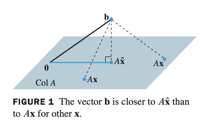
- $\mathbf{x}$ 는 $\mathbb{R}^m$ space 에 있으면 Col $A$ 에 존재한다.
$m \times n$ 크기인 행렬 $A$ 의 column 이 linearly independent 라는 말이 없으므로, dim Col $A \le n$ 이다. 왜냐하면 linearly independent 인 경우 dimension은 column vector 들인 n개 이기 때문이다. (dependent 할 경우 한단계 낮은 차원에서 표현이 가능하니깐..)
- $\mathbf{b}$ 와 가장 근접한 $\mathbf{x}$ 를 찾았다고 가정하고 이를 $\widehat{\mathbf{x}}$ 라고 표현하면
- $A\widehat{\mathbf{x}} = \widehat{\mathbf{b}}$ 으로 표현할 수 있다.
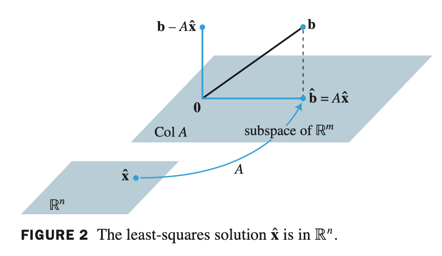
- $\widehat{\mathbf{b}}$ 은 $\mathbb{R}^n$ space 에 존재하고 matrix $A$ 에 의해서 linear transformation 된 결과가 $\widehat{\mathbf{x}}$ 이다.
- 여기서 $\widehat{\mathbf{b}}$ 이 Col $A$ 에 존재하는데, 이는 $A\widehat{\mathbf{x}} = \widehat{\mathbf{b}}$ 은 consistent 하다는 의미, 즉 해가 존재한다는 의미이다.
만약 free variable 을 지니게 되면 해가 무수히 많다.
- 여기서 Col $A$ 와 $\mathbf{b} - A\widehat{\mathbf{x}}$ 둘 의 관계는 orthogonal 하다. 따라서 $A = [\mathbf{a}_1 \quad \dots \quad \mathbf{a}_n]$ 으로 표현한다면 다음과 같은 식이 성립한다.
- 따라서 정의는 $\mathbf{a}_k$ 의 transpose를 multiplication 한 것과 같으므로
- 풀어서 쓰면
- 식을 정리하면
- 위 식은 $\mathbf{x}$ 가 least-squares solution of $A\mathbf{x} = \mathbf{b}$ 일 때 만족한다.
- 위 식을 정규 방정식 (normal equation) 이라고 한다.
- 최종적으로 $\widehat{\mathbf{x}}$ 을 찾기 위해 normal equation 을 풀면된다.
Theorem13.
The set of least-squares solutions of $\; A\mathbf{x} = \mathbf{b} \;$ coincides with the nonempty set of solutions of the normal equations $\; A^TA\mathbf{x} = A^T\mathbf{b}$ .
- normal equation 의 해 nonempty 집합은 $A\mathbf{x} = \mathbf{b}$ 의 least-squares solution 과 일치한다. least-squares solution 은 $\widehat{\mathbf{x}}$ 을 의미한다.
- $\widehat{\mathbf{x}}$ 은 normal equation 을 풀면 구할 수 있다.
- 증명
- $\mathbf{b} - A\widehat{\mathbf{x}}$ 은 $A$ 의 column set 인 Col $A$ 와 orthogonal 하다.
- 그리고 $A\widehat{\mathbf{x}}$ 은 Col $A$ 에 존재한다.
- 위 두개를 이용하여 우리는 저번 포스팅에서 공부했던 직교 분해(orthogonal decomposition) 로 표현할 수 있다. $\; \mathbf{y} = \widehat{\mathbf{y}} + \mathbf{z}$
- 여기서 $\mathbf{b}$ 의 decomposition 은 unique 하다는 것을 배웠다.
- $A\widehat{\mathbf{x}}$ 은 $\mathbf{b}$ 를 Col $A$ 에 orthogonal projection 한 것이고, $(\mathbf{b} - A\widehat{\mathbf{x}})$ 은 $\mathbf{b}$ 의 직교 요소이다.
- 따라서 $A\widehat{\mathbf{x}} = \widehat{\mathbf{b}}$ 에서 $\widehat{\mathbf{x}}$ 은 least-squares solution 이다.
Least-Squares Error - 최소 자승 에러
When a least-squares solution $\; \widehat{\mathbf{x}} \;$ is used to produce $\; A\widehat{\mathbf{x}} \;$ as an approximation to $\mathbf{b}$ , the distance from $\mathbf{b}$ to $\; A\widehat{\mathbf{x}} \;$ is called least-squares error of this approximation.
- $\mathbf{b}$ 에 근사치로서 $\; A\widehat{\mathbf{x}} \;$ 를 만들기 위해 least-squares solution 인 $\widehat{\mathbf{x}}$ 이 사용되면, $\mathbf{b}$ 와 $\; A\widehat{\mathbf{x}} \;$ 의 거리는 근사치의 least-squares error 라고 한다.
Example 1
\[A = \begin{bmatrix} 4 & 0 \\\ 0 & 2 \\\ 1 & 1 \end{bmatrix} \;, \quad \mathbf{b} = \begin{bmatrix} 2 \\\ 0 \\\ 11 \end{bmatrix}\]
Find a least-squares solution of the inconsistent system $\; A\mathbf{x} = \mathbf{b}$ for
- normal equation 을 찾으면 된다. $ \; A^TA\mathbf{x} = A^T\mathbf{b} $
- (1) augmented matrix 로 만들고 row reduction 으로 least-squares solution 구하기
- $A^TA$ 와 $A^T\mathbf{b}$ 두 개를 augmented matrix 로 만들어주고 row reduction 을 하면 다음과 같다.
- augmented matrix 의 제일 우측 column은 general solution 이므로 $ x_1 = 1 \quad x_2 = 2 $ 가 되므로..
- (2) augmented matrix 로 만들고 determinant 가 0이 아님을 이용하여 inverse matrix 로 구하기
- $A^TA$ 의 determinant 가 0이 아니고 $2 \times 2$ matrix 이므로 inverse 를 직접 구하면
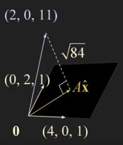
- least-squares error 를 구해보자
- 기히학적으로 표현해보면 다음과 같다.
- A 의 column space (4,0,1) (0,2,1) 두 개를 span 하여 subspace 를 만들수 있다.
\[A^TA = \begin{bmatrix} 6 & 2 & 2 & 2 \\\ 2 & 2 & 0 & 0 \\\ 2 & 0 & 2 & 0 \\\ 2 & 0 & 0 & 2 \end{bmatrix}\] \[A^T\mathbf{b} = \begin{bmatrix} 4 \\\ -4 \\\ 2 \\\ 6 \end{bmatrix}\]Example 2
\[A = \begin{bmatrix} 1 & 1 & 0 & 0 \\\ 1 & 1 & 0 & 0 \\\ 1 & 0 & 1 & 0 \\\ 1 & 0 & 1 & 0 \\\ 1 & 0 & 0 & 1 \\\ 1 & 0 & 0 & 1 \end{bmatrix} \;, \quad \mathbf{b} = \begin{bmatrix} -3 \\\ -1 \\\ 0 \\\ 2 \\\ 5 \\\ 1 \end{bmatrix}\]
Find a least-squares solution of the inconsistent system $\; A\mathbf{x} = \mathbf{b}$ for
- augmented matrix 로 조합하여 row reduction 을 진행해보면..
- 여기서 $\widehat{\mathbf{x}}$ 이 free variable 을 가지고 있는 general solution 이 나올 수 있지만, $A\widehat{\mathbf{x}}$ 를 계산해주면 반드시 단일 벡터 값이 나온다.
실제로 계산해보면 $\mathbf{x}_4$ 는 전부 사라지고 없다. 만약 $A\widehat{\mathbf{x}}$ 를 계산한 값에 단일 벡터 point 에 대한 값이 얻어지지 않고 free variable 이 포함된 general solution 이 얻어졌다면 계산 과정에서 실수가 있다는 것이다.
- 마지막으로 least-squares error 를 구해보면
Example 3
Let $A$ be an $m \times n$ matrix. Show that a vector $\mathbf{x}$ in $\mathbb{R}^n$ satisfies $A\mathbf{x} = \mathbf{0}$ if and only if $A^TA\mathbf{x} = \mathbf{0}$ .
- $A\mathbf{x} = \mathbf{0}$ 에다가 양변에 $A^T$ 를 multiplication 을 해주자.
- $A^T$ 를 0벡터에 multiplication 해도 결국 0벡터가 된다.
- 거꾸로도 한 번 생각해보자.
- 여기서 $\mathbf{x}^T$ 를 양변에 곱해준다.
- 위 식을 우리가 배운 성질에 의해서 다음과 같이 표현이 가능하다.
- 이 말은 곧 $A\mathbf{x}$ 의 length 가 0이라는 뜻이다. $ \lVert A\mathbf{x} \rVert = 0$
따라서, 벡터의 모든 entry 가 0이므로 $A\mathbf{x} = \mathbf{0}$ 을 만족한다.
- 또한 $\mbox{Nul} A = \mbox{Nul} A^TA $ 를 만족한다.
\[A^TA\mathbf{x} = \mathbf{0}\]Example 4
Let $A$ be an $m \times n$ matrix such that $A^TA$ is invertible. Show that the columns of $A$ are linearly independent.
- 위 식에서 $A^TA$ 란 말은 결국 $A$ 는 square matrix 라는 말이다. 만약, square matrix 가 invertible 하다면, trivial solution 를 갖는다.
- trivial solution 을 갖으면 다음 homogeneous equation 을 만족한다.
- 위 식은 matrix $A$ 의 column vector 들이 모두 linearly independent 하다는 의미이기도 하다.
Example 5
Let $A$ be an $m \times n$ matrix whose columns are linearly independent.
a. Show that $A^TA$ is invertible.
b. Explain why $m \ge n$ .
c. Determine the rank of $A$ .
- (a.) 를 확인해보자.
- linearly independent 하다고 주어졌으므로 다음 식이 성립한다.
- 이말은 has only trivial solution, 즉 trivial solution 만을 갖는다는 의미이고 양변에 $A^T$ 를 곱해주면 된다.
- 0벡터에 $A^T$ multiplication 을 해도 결국 0벡터이므로 다음 식을 만족한다.
- 따라서, trivial solution 을 갖는다면 $A^TA$ 는 square matrix 이고 invertible 하다는 뜻이다.
- (b.) 를 확인해보자.
- 문제에서 linearly independent 하다는 조건이 있으므로, matrix $A$ 는 $n$ 개의 linearly independent 한 column vector 들을 갖고 있다는 뜻이다.
- 여기서 m 은 n 보다 크거나 같아야 linearly independent 하다. 챕터 1.6 theorem 8 을 확인해보자.
- (c.) 를 확인해보자.
- rank 의 정의는 다음과 같다.
rank of $A = $ dim Col $A = n$
- 여기서 linearly independent 하므로 Col $A$ 의 dimension 은 $n$ 임을 만족한다.
Theorem14.
Let $A$ be an $m \times n$ matrix. The following statements are logically equivalent:
a. The equation $\; A\mathbf{x} = \mathbf{b} \;$ has a unique least-squares solution for each $\mathbf{b}$ in $\; \mathbb{R}^m$ .
b. The columns of $A$ are linearly independent.
c. The matrix $\; A^TA \;$ is invertible.When these statements are true, the least-squares solution $\widehat{\mathbf{x}}$ is given by
\[\widehat{\mathbf{x}} = (A^TA)^{-1}A^T\mathbf{b}\]
- a. $\; A\mathbf{x} = \mathbf{b} \;$ 는 $\mathbf{b}$ 에 대한 최소자승해는 유일하다.
- b. $A$ 의 column 들은 선형 독립이다.
- c. $A^TA$ 는 역행렬이 존재한다.
Theorem15.
Given an $m \times n$ matrix $A$ with linearly independent columns, let $\; A = QR \;$ be a QR factorization of $A$ as in Theorem 12. Then, for each $\mathbf{b}$ in $\mathbb{R}^m$ , the equation $\; A\mathbf{x} = \mathbf{b} \;$ has a unique least-squares solution, given by
\[\widehat{\mathbf{x}} = R^{-1}Q^T\mathbf{b}\]
- $A$ 가 선형 독립 column 으로 이루어져 있으면 $A$ 를 QR로 decomposition 할 수 있다는 것을 배웠었다.
- 여기서 Q는 orthonormal column 으로 이루어진 행렬이고, R은 upper triangular matrix 이다.
- $A$ 가 QR 분해가 가능한 행렬이면 최소자승해는 다음과 같이 구할 수 있다. $ \widehat{\mathbf{x}} = R^{-1}Q^T\mathbf{b} $
- 증명
- $A\widehat{\mathbf{x}} = \mathbf{b}$ 에 $A = QR$ 과 위 식을 대입하면 다음과 같이 된다.
- $Q$ 는 $A$ 의 orthonormal basis 이다.
- QQ^T 는 1이 되어 $A\widehat{\mathbf{x}} = \mathbf{b}$ 를 만족하게 된다.
- $\widehat{\mathbf{x}}$ 을 구해보면
- $\widehat{\mathbf{x}}$ 을 구할 때는
- 위 식보다는
- 이 식을 더 많이 사용한다. $R$ 의 역행렬을 계산하기 위해서는 많은 연산이 필요하기 때문이다.
Example 6
\[A = \begin{bmatrix} 1 & 3 & 5 \\\ 1 & 1 & 0 \\\ 1 & 1 & 2 \\\ 1 & 3 & 3 \end{bmatrix} \; , \quad \mathbf{b} = \begin{bmatrix} 3 \\\ 5 \\\ 7 \\\ -3 \end{bmatrix}\]
Find a least-squares solution of $A\mathbf{x} = \mathbf{b}$ for
- $\widehat{\mathbf{x}}$ 을 구하기 위해서는 $ R\widehat{\mathbf{x}} = Q^T\mathbf{b} $ 식을 풀면된다. 마찬가지로 augmented matrix 를 구성해서 row reduction 을 진행해준다.
Least-Squares Lines
- 우리가 어떤 실험을 통해서 $x$ 와 $y$ 라는 데이터군을 얻었다고 가정하자.
- 다음과 같이 $(x_1, y_1), (x_2, y_2), \dots , (x_n, y_n)$ $n$ 개의 데이터 포인트를 얻었다고 할 때 우리가 이 데이터군을 선형적인 관계에 있다고 가정해보자.
- 여기서 데이터군을 가장 잘 표현할 수 있는 $y = \beta _0 + \beta _1 x$ 라는 수식에 데이터군들을 least-squares method 를 사용해서 피팅을 하려고 한다.
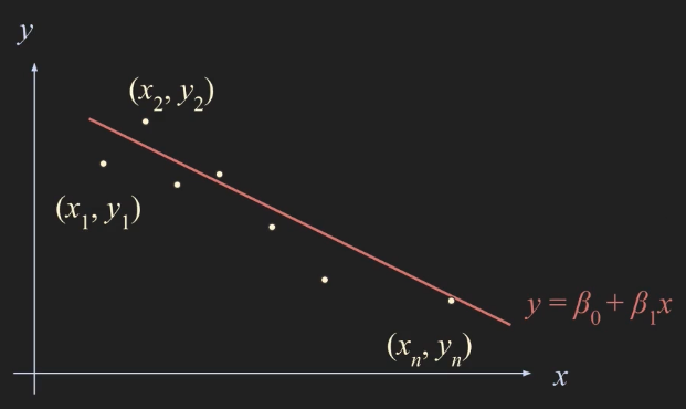
- 여기서 결정되지 않은 부분은 $\beta _0, \beta _1$ 이므로 다음과 같이 예측할 수 있다.
$x_n$ 까지의 관측된 값을 구하는 과정이다.
- Predicted $y$ - value Observed $y$ - value
$\beta _0 + \beta _1 x_1$ $=$ $y_1$
$\beta _0 + \beta _1 x_2$ $=$ $y_2$
$\vdots$ $\vdots$
$\beta _0 + \beta _1 x_n$ $=$ $y_n$ - 위 값들을 가지고 linear equation, matrix equation 으로 표현해보면
- 하지만 위 식을 만족하는 $\mathbf{\beta}$ 벡터는 없다. 즉 inconsistent 하다.
- 따라서 $\mathbf{y}$ 에 제일 가깝게 하는 length 혹은 norm 측면에서 제일 가깝게 하는 $\beta _0, \beta _1$ 값을 찾아야한다.
- 그 방법은 바로 least-squares method 의 normal equation 을 풀면 된다.
- 우리가 구하고자 하는 $\mathbf{\beta}$ 는 바로 least-squares solution 인 $\widehat{\mathbf{\beta}}$ 의 solution 이다.
Least-Squares Fitting of Other Curves
- 하지만 모든 데이터들이 위처럼 선형적으로 표현되지는 않는다. 다른 커브들에 대해서 어떻게 적용하는지 살펴보자.
- 만약 우리가 구하고자 하는 그래프가 2차방정식의 모양을 가진다면
데이터군이 위 수식처럼 표현된다면
- Predicted $y$ - value Observed $y$ - value
$\beta _0 + \beta _1 x_1 + \beta _2 x_1^2$ $=$ $y_1$
$\vdots$ $\vdots$
$\beta _0 + \beta _1 x_n + \beta _2 x_n^2$ $=$ $y_n$ - 위 값들을 가지고 linear equation, matrix equation 으로 표현해보면
- 마찬가지로 least-squares method 의 normal equation 을 통해 least-squares solution 을 구할 수 있다.
- 우리는 여태껏 polynomial equation 만 다뤘는데 만약 임의의 function 에 데이터군을 피팅하고 싶은 경우도 발생할 것이다.
- 임의의 function 에 피팅할 경우 다음과 같이 표현이 가능하다.
- 이 식을 matrix equation 으로 표현하면 다음과 같다.
- 마찬가지로 least-squares method 의 normal equation 을 통해 least-squares solution 을 구할 수 있다.
Weighted Least-Squares
- 우리가 지금까지 least-squares method 를 사용하여 어떤 그래프에 피팅하는 작업은 $\mathbf{y}, \widehat{\mathbf{y}}$ 두 개를 찾아서 둘 의 length 를 최소화하는 방법이였다.
- 하지만, 때로는 데이터에 따라 특별히 가중치를 두고 싶은 경우가 발생한다. 어떤 데이터는 큰 가중치값을, 작은 가중치값을 적용한다고 하면 error 를 구하는 식이 다음과 같이 표현가능하다.
- 가중치가 위와 같으면 length 는 다음과 같이 표현할 수 있다.
- 정리하자면 least-squares solution 을 구하는 방법은 다음과 같다.