
Linear Algebra - 5.4 The Gram-Schmidt Process (그람 슈미츠 과정)

- Linear Algebra - 1.1 Systems of Linear Equations
- Linear Algebra - 1.2 Row Reduction and Echelon Forms
- Linear Algebra - 1.3 Vector Equations
- Linear Algebra - 1.4 The Matrix Equation Ax=b
- Linear Algebra - 1.5 Solution Sets of Linear Systems
- Linear Algebra - 1.6 Linear Independence and Linear Dependence
- Linear Algebra - 1.7 Introduction to Linear Transformation
- Linear Algebra - 1.8 The Matrix of a Linear Transformation
- Linear Algebra - 2.1 Matrix Operations
- Linear Algebra - 2.2 The Inverse of Matrix
- Linear Algebra - 2.3 Characterizations of Invertible Matrices of
- Linear Algebra - 2.4 Partitioned Matrices
- Linear Algebra - 2.5 Matrix Factorizations, LU Decomposition
- Linear Algebra - 2.6 Subspaces of $\mathbb{R}^n$
- Linear Algebra - 2.7 Dimension and Rank
- Linear Algebra - 3.1 Introduction to Determinants
- Linear Algebra - 3.2 Properties of Determinants
- Linear Algebra - 3.3 Cramer's Rule, Volume, And Linear Transformations
- Linear Algebra - 4.1 Eigenvectors and Eigenvalues
- Linear Algebra - 4.2 The Characteristic Equation
- Linear Algebra - 4.3 Diagonalization
- Linear Algebra - 4.4 Eigenvectors And Linear Transformations
- Linear Algebra - 4.5 Complex Eigenvalues
- Linear Algebra - 5.1 Inner Product And Orthogonality
- Linear Algebra - 5.2 Orthogonal Sets
- Linear Algebra - 5.3 Orthogonal Projections
- Linear Algebra - 5.4 The Gram-Schmidt Process (그람 슈미츠 과정)
- Linear Algebra - 5.5 Least-Square Problems
- Linear Algebra - 6.1 Diagonalization of Symmetric Matrices
- Linear Algebra - 6.2 Quadratic Forms
- Linear Algebra - 6.3 Constrained Optimization
- Linear Algebra - 6.4 SVD, The Singular Value Decomposition
- Linear Algebra - 6.5 Reduced SVD, Pseudoinverse, Matrix Classification, Inverse Algorithm

용어 정리
- Gram-Schmidt Process - 그람-슈미츠 과정
- QR factorization - QR 분해
- 그람 슈미트 과정은 임의의 subspace 가 있을 때, 그 subspace 를 이루는 orthogonal basis 를 찾는 방법이다.
Basis idea for the Gram-Schmidt process - 그람 슈미트 과정의 기본 아이디어
- {$\mathbf{u}_1 , \mathbf{u}_2$} is a basis for $W = $ Span{$\mathbf{u}_1 , \mathbf{u}_2$} 이라고 가정하자.
- dim = 2 이고 2차원 공간이다.
- 그렇다면 $\mathbf{u}_1 , \mathbf{u}_2$ 는 서로 linearly independent 한 관계에 있다.
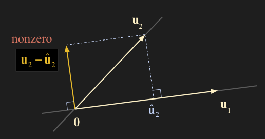
여기서 우리는 subspace W 에 대한 orthogonal basis {$\mathbf{v}_1 , \mathbf{v}_2$} 를 찾을 수 있다.
- 먼저 $\mathbf{v}_1$ 을 $\mathbf{u}_1$ 과 같다고 가정해보면
- $\mathbf{v}_1$ 은 subspace W 에 있다.
- $\mathbf{v}_2$ 도 마찬가지로 subspace W 에 있는데, 이유는 $\mathbf{v}_2$ 는 결국 $\mathbf{u}_1, \mathbf{u}_1$ 의 linear combination 으로 표현이 가능하기 때문이다.
- 여기서 $\mathbf{v}_1, \mathbf{v}_2$ 는 nonzero 이고 orthogonal 하기 때문에 linearly independent set 이고 다음과 같이 표현이 가능하다.
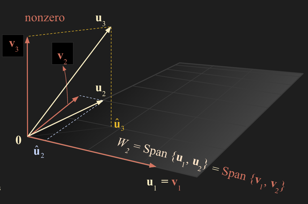
- {$\mathbf{u}_1 , \mathbf{u}_2 , \mathbf{u}_3 $} is a basis for $W = $ Span{$\mathbf{u}_1 , \mathbf{u}_2 , \mathbf{u}_3 $} 이라고 가정하자.
- dim = 3 이고 3차원 공간이다.
- 그렇다면 위와 마찬가지로 $\mathbf{u}_1 , \mathbf{u}_2$ 는 서로 linearly independent 한 관계에 있고 $\mathbf{u}_1 , \mathbf{u}_2$ 를 span 하는 subspace $W_2$ 를 그림과 같이 가정해보자.
- $\mathbf{u}_3$ 를 subspace $W_2$ 에 대해 orthogonal projection 한 $\widehat{\mathbf{u}}_3$ 를 가정하면 다음과 같은 식을 도출할 수 있다.
- 여기서 $\mathbf{v}_3$ 는 $\mathbf{u}_1, \mathbf{u}_2$ 를 span 하는 subspace $W_2$ 에 닫혀있으므로 $\mathbf{v}_3$ 는 $\mathbf{u}_1, \mathbf{u}_1$ 의 linear combination 형태로 표현가능하므로 linearly independent 하다. 또한 $\mathbf{v}_1, \mathbf{v}_2, \mathbf{v}_3$ 는 각각 orthogonal 한 관계에 있다.
- 여기서 2차원 2개, 3차원 3개만 과정을 수행하는게 아니라 계속 무한히 늘려나가는 과정을 정리한 것이 그람 슈미트 과정이다.
- 위 과정을 일반화한 정리이다.
Theorem11. The Gram-Schmidt Process
Given a basis {$\mathbf{x}_1 , \dots , \mathbf{x}_p$} for a nonzero subspace $W$ of $\; \mathbb{R}^n \;$ , define
\[\mathbf{v}_1 = \mathbf{x}_1\] \[\mathbf{v}_2 = \mathbf{x}_2 - {\mathbf{x}_2 \cdot \mathbf{v}_1 \over \mathbf{v}_1 \cdot \mathbf{v}_1 } \mathbf{v}_1\] \[\mathbf{v}_3 = \mathbf{x}_3 - {\mathbf{x}_3 \cdot \mathbf{v}_1 \over \mathbf{v}_1 \cdot \mathbf{v}_1 } \mathbf{v}_1 - {\mathbf{x}_3 \cdot \mathbf{v}_2 \over \mathbf{v}_2 \cdot \mathbf{v}_2 } \mathbf{v}_2\] \[\vdots\] \[\mathbf{v}_p = \mathbf{x}_p - {\mathbf{x}_p \cdot \mathbf{v}_1 \over \mathbf{v}_1 \cdot \mathbf{v}_1 } \mathbf{v}_1 - {\mathbf{x}_p \cdot \mathbf{v}_2 \over \mathbf{v}_2 \cdot \mathbf{v}_2 } \mathbf{v}_2 - \dots - { \mathbf{x}_p \cdot \mathbf{v}_{p-1} \over \mathbf{v}_{p-1} \cdot \mathbf{v}_{p-1} } \mathbf{v}_{p-1}\]Then {$\mathbf{v}_1 , \dots , \mathbf{v}_p $} is an orthogonal basis for $W \; $ . In addition
Span ${\mathbf{v}_1 , \dots , \mathbf{v}_k}$ = Span {$\mathbf{x}_1 , \dots , \mathbf{x}_k$} $\quad \quad$ $\mbox{for} \; \le \; k \; \le \; p $
\[\mathbf{v}_1 = \mathbf{x}_1 = \begin{bmatrix} 3 \\\ 6 \\\ 0 \end{bmatrix}\] \[\mathbf{v}_2 = \mathbf{x}_2 - {\mathbf{x}_2 \cdot \mathbf{v}_1 \over \mathbf{v}_1 \cdot \mathbf{v}_1 } \mathbf{v}_1 = \begin{bmatrix} 1 \\\ 2 \\\ 2 \end{bmatrix} - {15 \over 45} \begin{bmatrix} 3 \\\ 6 \\\ 0 \end{bmatrix} = \begin{bmatrix} 0 \\\ 0 \\\ 2 \end{bmatrix}\]Example 1
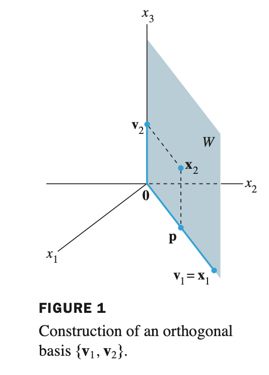
Let $W =$ Span {$\mathbf{x}_1, \mathbf{x}_2$}, where $\mathbf{x}_1 = (3, 6, 0) \; , \; \mathbf{x}_2 = (1, 2, 2)$ . Construct an orthogonal basis {$\mathbf{v}_1, \mathbf{v}_2$} for $W$ .
- $\mathbf{v}_2$ 는 $\mathbf{v}_1$ 과 orthogonal 하므로 $W$ 에 대한 orthogonal basis 를 만든 것이다.
Example 2
Let $W =$ Span {$\mathbf{x}_1, \mathbf{x}_2, \mathbf{x}_3$}, where $\mathbf{x}_1 = (1, 1, 1, 1) \; , \; \mathbf{x}_2 = (0, 1, 1, 1) \; , \; \mbox{and} \; \mathbf{x}_3 = (0, 0 , 1, 1)$ . Construct an orthogonal basis for $W$ .
- {$\mathbf{x}_1, \mathbf{x}_2, \mathbf{x}_3$} is a linearly independent set
- $\mathbf{v}_2$ 는 $\mathbf{x}_2$ 에 $\mathbf{x}_2$ 를 $\mathbf{x}_1$ 에 projection 한 것을 빼서 구할 수 있다.
- $\mathbf{v}_2$ 는 $\mathbf{x}_1$ 에 직교한 $\mathbf{x}_2$ 의 요소이므로, {$\mathbf{v}_1, \mathbf{v}_2 $} 는 $W$ 에 대한 orthogonal basis 라고 할 수 있다.
- 여기서 $\mathbf{v}_2$ 에 4를 곱하는 스케일링을 통해 $\mathbf{v}^{\prime}_2$ 을 만들어주자.
- $\mathbf{x}_3$ 를 2차원 $W$ 에 projection 한 것은 $W$ 를 span 하는 각각의 orthogonal basis 에 projection 한 뒤 그것들을 더해주면 된다.
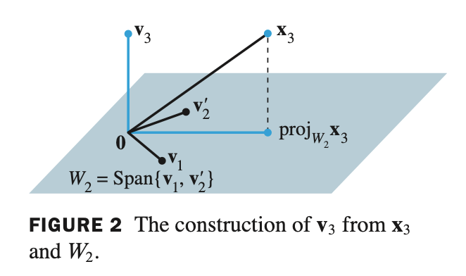
- 이제 $\mathbf{v}_1, \mathbf{v}_2, \mathbf{v}_3$ 가 $W$ 를 span 하는 orthogonal basis 가 된다.
Orthonormal Basis - 정규직교 기저
- orthonormal basis 는 orthogonal basis 로 부터 손쉽게 구할 수 있다. 단순히 orthogonal basis 들을 normalize 를 해주면 된다.
- normalize 는 벡터의 길이가 1이 되도록 하는 방법이다.
\[\mathbf{v}_1 = \begin{bmatrix} 3 \\\ 6 \\\ 0 \end{bmatrix} \quad \quad \mathbf{v}_2 = \begin{bmatrix} 0 \\\ 0 \\\ 2 \end{bmatrix}\] \[\mathbf{u}_1 = {\mathbf{v}_1 \over \lVert \mathbf{v}_1 \rVert} = \begin{bmatrix} 1 / \sqrt{5} \\\ 2 / \sqrt{5} \\\ 0 \end{bmatrix} \quad \quad \mathbf{u}_2 = {\mathbf{v}_2 \over \lVert \mathbf{v}_2 \rVert} = \begin{bmatrix} 0 \\\ 0 \\\ 1 \end{bmatrix}\]Example 3
Let $W =$ Span {$\mathbf{x}_1, \mathbf{x}_2$}, where $\mathbf{x}_1 = (3, 6, 0), \mathbf{x}_2 = (1, 2, 2)$ . Construct an orthonormal basis {$\mathbf{u}_1, \mathbf{u}_2$} for $W$ .
QR Factorization Matrices - 행렬의 QR 분해
The QR Factorization
If $A$ is an $m \times n$ matrix with linearly independent columns, then $A$ can be factored as $\; A = QR \;$ , where $Q$ is an $m \times n$ matrix whose columns form an orthonormal basis for Col $A$ and $R$ is an $n \times n$ upper triangular invertible matrix with positive entries on its diagonal.
column 이 linearly independent 한 $m \times n$ 크기의 행렬 $A$ 는 $A = QR$ 로 분해될 수 있다.
여기서 $Q$ 는 column 이 Col $A$ 에 대한 orthonormal basis 로 이루어진 $m \times n$ 크기의 행렬이고, $R$ 은 $n \times n$ 크기의 모든 diagonal entries 가 양수를 가진 upper triangular invertible matrix 이다.
- 증명
- $A$ 의 column 이 Col $A$ 에 대한 기저 {$\mathbf{x}_1 , \dots , \mathbf{x}_n$} 으로 구성되어 있다.
- $W = $ Col $A$ 에 대한 orthogonal basis {$\mathbf{u}_1 , \dots , \mathbf{u}_n$} 를 구하기 위해서 그람슈미트 과정을 사용한다.
- 이후 그람 슈미트 과정으로 구한 orthogonal basis 를 orthonormal basis 로 변형시키면 $Q$ 를 구할 수 있다.
- Col $A$ 의 basis $\mathbf{x}$ 는 Col $A$ 의 orthonormal basis $\mathbf{u}$ 의 linear combination 으로 표현 할 수 있다.
- 이것은 $\mathbf{x}_k$ 가 $Q$ 의 column 들의 선형 결합으로 나타낼 수 있다는 의미이다.
- 각각의 가중치(weight) 들을 벡터로 표현하면 다음과 같다.
- $\mathbf{x}$ 는 $Q$ 와 weight $r$ 로 표현할 수 있으므로 다음과 같은 식이 성립한다.
- 여기서 $R$ 은 invertible 하고 다음과 같이 나타낼 수 있다
$A\mathbf{c} = 0$ 은 trivial solution 이다.
최종적으로 $R$ 의 모습
QR Factorization Steps - QR 분해 단계
(1)
Gram-Schmidt 과정으로 Col $A$ 에 대한 orthonormal basis 를 찾는다. 이것이 $Q$ 가 된다.
(2)
\[Q^TA = Q^T(QR) = IR = R\]
$R$ 은 다음과 같이 찾을 수 있다.$Q$ 는 orthonormal basis 의 column 을 지니고 있으므로, $Q^TQ$ 는 $Q$ 의 길이를 의미한다. orthonormal basis 의 길이는 1 이므로, $Q$ 의 길이도 1이 된다. 따라서 identity matrix 인 $I$ 가 된다.
(3)
If $r_{kk} < 0$ , switch the sign of \(\mathbf{u}_k \; (- \mathbf{u}_k)\) and \(r_{kk}\) to \(r_{kn}\)만약 $R$ 의 diagonal entry 인 $r_{kk}$ 가 음수이면, \(\mathbf{u}_k\) 의 부호를 바꾸고 \(r_{kk}, r_{kn}\) 의 부호를 바꿔준다.
\[\mathbf{v}_1 = \begin{bmatrix} 1 \\\ 1 \\\ 1 \\\ 1 \end{bmatrix} \; , \quad \mathbf{v}^{\prime}_2 = \begin{bmatrix} -3 \\\ 1 \\\ 1 \\\ 1 \end{bmatrix} \; , \quad \mathbf{v}_3 = \begin{bmatrix} 0 \\\ -2/3 \\\ 1/3 \\\ 1/3 \end{bmatrix}\] \[Q = \begin{bmatrix} 1/2 & -3 / \sqrt{12} & 0 \\\ 1/2 & 1 / \sqrt{12} & -2 / \sqrt{6} \\\ 1/2 & 1 / \sqrt{12} & 1 / \sqrt{6} \\\ 1/2 & 1 / \sqrt{12} & 1 / \sqrt{6} \end{bmatrix}\] \[Q^TA = Q^T(QR) = IR = R\] \[R = \begin{bmatrix} 1/2 & 1/2 & 1/2 & 1/2 \\\ -3/\sqrt{12} & 1/\sqrt{12} & 1/\sqrt{12} & 1/\sqrt{12} \\\ 0 & -2/\sqrt{6} & 1/\sqrt{6} & 1/\sqrt{6} \end{bmatrix} \begin{bmatrix} 1 & 0 & 0 \\\ 1 & 1 & 0 \\\ 1 & 1 & 1 \\\ 1 & 1 & 1 \end{bmatrix}\] \[= \begin{bmatrix} 2 & 3/2 & 1 \\\ 0 & 3/\sqrt{12} & 2/\sqrt{12} \\\ 0 & 0 & 2/\sqrt{6} \end{bmatrix}\]Example 4
Find a $QR$ factorization of \(A = \begin{bmatrix} 1 & 0 & 0 \\\ 1 & 1 & 0 \\\ 1 & 1 & 1 \\\ 1 & 1 & 1 \end{bmatrix}\)