Linear Algebra - 4.5 Complex Eigenvalues

- Linear Algebra - 1.1 Systems of Linear Equations
- Linear Algebra - 1.2 Row Reduction and Echelon Forms
- Linear Algebra - 1.3 Vector Equations
- Linear Algebra - 1.4 The Matrix Equation Ax=b
- Linear Algebra - 1.5 Solution Sets of Linear Systems
- Linear Algebra - 1.6 Linear Independence and Linear Dependence
- Linear Algebra - 1.7 Introduction to Linear Transformation
- Linear Algebra - 1.8 The Matrix of a Linear Transformation
- Linear Algebra - 2.1 Matrix Operations
- Linear Algebra - 2.2 The Inverse of Matrix
- Linear Algebra - 2.3 Characterizations of Invertible Matrices of
- Linear Algebra - 2.4 Partitioned Matrices
- Linear Algebra - 2.5 Matrix Factorizations, LU Decomposition
- Linear Algebra - 2.6 Subspaces of $\mathbb{R}^n$
- Linear Algebra - 2.7 Dimension and Rank
- Linear Algebra - 3.1 Introduction to Determinants
- Linear Algebra - 3.2 Properties of Determinants
- Linear Algebra - 3.3 Cramer's Rule, Volume, And Linear Transformations
- Linear Algebra - 4.1 Eigenvectors and Eigenvalues
- Linear Algebra - 4.2 The Characteristic Equation
- Linear Algebra - 4.3 Diagonalization
- Linear Algebra - 4.4 Eigenvectors And Linear Transformations
- Linear Algebra - 4.5 Complex Eigenvalues
- Linear Algebra - 5.1 Inner Product And Orthogonality
- Linear Algebra - 5.2 Orthogonal Sets
- Linear Algebra - 5.3 Orthogonal Projections
- Linear Algebra - 5.4 The Gram-Schmidt Process (그람 슈미츠 과정)
- Linear Algebra - 5.5 Least-Square Problems
- Linear Algebra - 6.1 Diagonalization of Symmetric Matrices
- Linear Algebra - 6.2 Quadratic Forms
- Linear Algebra - 6.3 Constrained Optimization
- Linear Algebra - 6.4 SVD, The Singular Value Decomposition
- Linear Algebra - 6.5 Reduced SVD, Pseudoinverse, Matrix Classification, Inverse Algorithm

용어 정리
- conjugate - 짝으로 결합한 , 켤례
- conjugate complex numbers - 켤례복소수
Matrix Eigenvalue-Eigenvector Theory for $\mathbb{C}^n$ - 복소수 공간에서 행렬의 고유치-고유벡터 이론
- 우린 여태껏 $\mathbb{R}^n$ 공간, 즉 실수 공간에서의 고유값-고유벡터를 살펴보았다. 그렇다면 복소수 공간인 $\mathbb{C}^n$ 에서는 어떨까?
- 사실 실수 공간에 있는 이론이 그대로 다 적용이 된다. 단지 eigenvalue 가 complex value 를 갖게 될 뿐이다.
A complex scalar $\lambda \;$ satisfies $\mbox{det} \; (A - \lambda I) = 0$
if and only if there is a nonzero vector $\mathbf{x} \; $ in $\mathbb{C}^n \;$ such that $A\mathbf{x} = \lambda \mathbf{x}$복소수 scalar $\lambda \;$ 가 $\mbox{det} \; (A - \lambda I) = 0 \;$ 을 만족하면 $A\mathbf{x} = \lambda \mathbf{x} \; $ 에서 $\mathbb{C}^n \;$ space 에 존재하는 nonzero vector $\mathbf{x} \; $ 가 존재한다.
- 예시 문제1
- $A$ 가 다음과 같이 주어졌을 때, $A$ 의 eigenvalue 는 다음과 같다.
- characteristic equation 으로 $\lambda$ 를 구할 수 있다.
- 여기서 $\lambda = i, -i$ 가 되고 이는 conjugate(켤례 복소수) 관계에 있게된다.
- eigenvalue 에 해당되는 eigenvector 를 구하면 다음과 같다.
여기서 eigenvector 도 conjugate 관계에 있다.
이처럼 eigenvalue 와 eigenvector 에서 complex 부분이 conjugate 관계에 있다는 특징을 확인할 수 있다.
- 예시 문제2
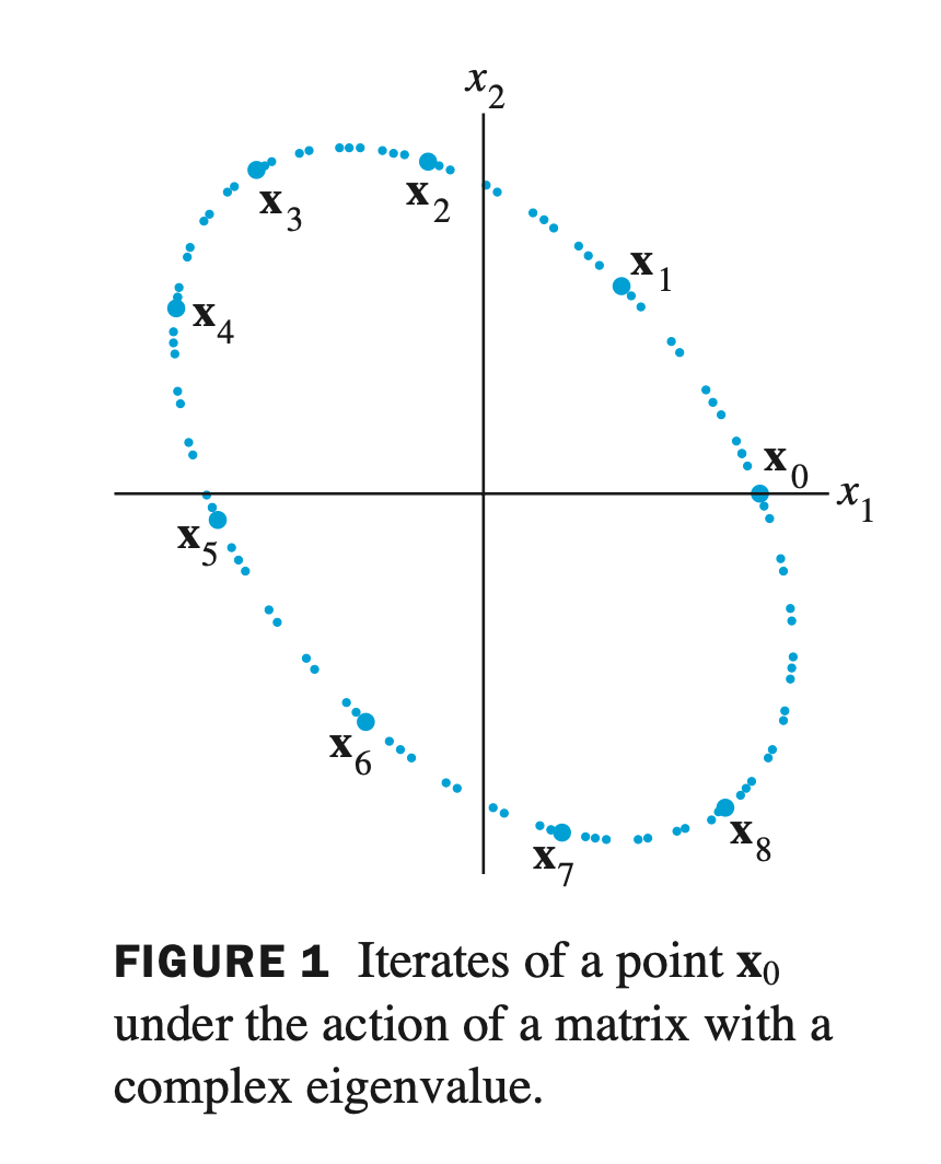
- complex eigenvalue 가 존재하는 행렬 $A$ 로 linear transformation 을 했을 때, 기하학적으로 어떻게 변하는지 파악해보자.
- $A$ 가 위와 같이 주어졌을 때 eigenvalue 를 찾고 eigenspace 에서의 basis를 찾아보자. 우선, $A$ 의 characteristic equation 으로 eigenvalue 를 찾는다.
- $A - \lambda I$ 로 eigenvalue 에 해당하는 eigenvector 를 찾을 수 있다.
- row reduction 을 통해 general solution 을 구하자.
- 여기서 두 가지 방법이 존재하는데, 첫번째는 정직하게 row reduction 을 푸는 행위인데, 여기서는 분수와 복소수가 존재하기 때문에 계산실수가 발생할 수도 있으니 다음과 같은 방법을 싸보자.
- 결과로 나온 행렬을 선형방정식으로 풀어서 표현하면 다음과 같다.
- 여기서 x_1 의 coefficient 로 복소수가 없는 두 번째 식을 $x_1$ 을 기준으로 general solution 을 표현하면 다음과 같다.
- $x_2 = 5$ 일 때 $\; x_1 = -2 -4i$ 가 된다.
- 이것이 $\lambda = 0.8 - 0.6i$ 일 때의 eigenvector 이다.
- 또한 $\lambda = 0.8 - 0.6i$ 일 때의 eigenvector 는 conjugate 관계에 있으므로 다음과 같다.
- $x = (2,0)$ 일 때 $A\mathbf{x}$ 를 반복수행하면 다음과 같다.
- 이것을 기하학적으로 표현하면 다음과 같다.
- 타원 형태가 나타난다. 이것이 complex eigenvalue 의 특성이다.
Eigenvalue and Eigenvectors of Real Matrix That Acts on $\mathbb{C}^n$ - 복소수 공간에서 작동하는 실수 행렬의 고유치와 고유벡터
- entires 가 real 인 $n \times n$ 행렬 $A$ 가 있을 때, $\lambda$ 가 complex space 에 존재하면 다음 식이 성립한다.
여기서 $\overline{A} , \overline{\mathbf{x}} , \overline{\lambda}$ 는 conjugate 를 의미한다.
행렬 $A$ 에 complex eigenvalue 가 주어지면 complex 의 conjugate 도 eigenvalue 가 되고 그에 해당하는 conjugate vector 도 eigenvector 가 된다.
When $A$ is real, its complex eigenvalues occur in conjugate pairs.
$A$ 가 real 일 때, $A$ 의 complex eigenvalues 는 conjugate pair 이다.
- 예시 문제 1
- $C$ 가 다음과 같이 주어졌을 때, 이것의 eigenvalue 와 $C$ 로 인한 transformation 이 어떻게 작동되는지 확인해보자.
- $C$ 의 eigenvalues 는 다음과 같다.
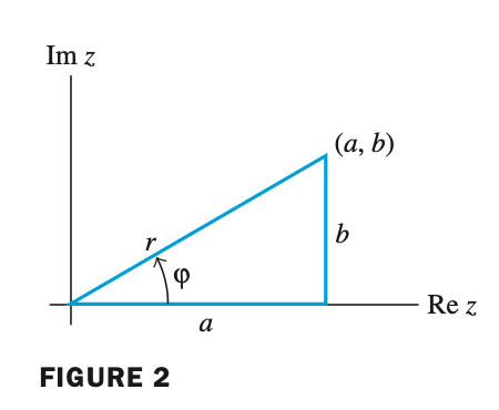
- $C$ 를 다음과 같이 표현할 수 있다.
- $r = \sqrt{a^2 + b^2}$ 이며, 이는 transformation 을 했을 때 scaling 한 값이 된다.
- 이제 complex eigenvalue 를 갖는 행렬 $C$ 로 $x$ 를 transformation 하면 다음과 같다.
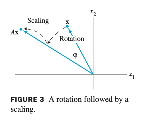
- rotation 과 scaling 이 된것을 확인할 수 있다. a 와 b 에 따라서 scaling 크기가 다르다.
- 예시 문제 2
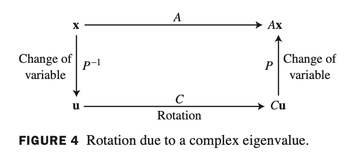
complex eigenvalue 를 갖고 있는 행렬 $A$ 는 eigenvalue 의 real part 와 imaginary part 로 구성된 행렬 $C$ 와 similar 관계에 있다.
- 행렬 $A$ 가 다음과 같이 주어졌을 때, eigenvalue 와 eigenvector 를 구해보자.
- $A$ 와 similar 관계에 있는 matrix 를 찾기 위해 $P$ 를 다음과 같이 구할 수 있다.
- 이제 $C = P^{-1}AP $ 를 해보면 $A$ 와 similar 관계에 있는 행렬 $C$ 를 구할 수 있다.
- $C$ 의 entries 는 eigenvalue 의 real part 와 imaginary part 가 된다. 또한 $C$ 행렬으로 transformation 을 적용하면 $r = 1$ 이므로 순수한 회전 동작만 작동한다.
Theorem8.
Let $A$ be a real $2 \times 2 \;$ matrix with a complex eigenvalue $\lambda = a - bi \; (b \ne 0) \;$ and an associated eigenvector $\mathbf{v} \;$ in $\mathbb{C}^2$ . Then
$A = PCP^{-1} \; , \quad \mbox{where} \quad P = [\mbox{Re} \; \mathbf{v} \quad \mbox{Im} \; \mathbf{v}] \quad \mbox{and} \quad C = \begin{bmatrix} a & -b \\ b & a \end{bmatrix} $
- $P$ 는 eigenvector 의 real part, imaginary part 가 되고 $C$ 는 eigenvalue 의 real part, imaginary part 가 된다.
- 증명
- 우선 $\mbox{Re} \; \mathbf{v}$ 와 $\mbox{Im} \; \mathbf{v}$ 가 linearly dependent 라고 가정하고 임의의 벡터 $\mathbf{u}$ 가 존재한다고 하면
- $\mathbf{v}$ 벡터를 conjugate pair 로 나타내면
- 여기에 각각 해당되는 eigenvalue 는 다음과 같다.
- $A\mathbf{v} = \lambda \mathbf{v}$ 성질을 이용하면 다음과 같이 나타낼 수 있다.
- 여기서 위의 두개의 conjugate pair 를 더해보면
- (i) $c = 0$ 인 경우
- $c$ 가 0이면 $ 0 = - b\mathbf{u}$ 가 되고 여기서 $\mathbf{u}$ 는 nonzero vector 이기 때문에 $b = 0$ 이 되어야한다.
- 하지만, $b = 0$ 이면 eigenvalue $\lambda = a + 0i = a$ 가 되어버리고 이는 eigenvalue 가 real value 실수라는 의미이다.
- complex space 에서 eigenvalue 가 real value 인것은 매우 모순적이므로, $c$ 가 0이 되어서는 안된다.
- (ii) $c \ne 0$ 인 경우 다음과 같이 정리할 수 있다.
- 여기서 $\mathbf{u}$ 는 real vector 이고, ${ (ac - b) \over c }$ 는 scalar 값이다.
- 이말인즉슨, $A$ 의 eigenvalue 는 ${ (ac - b) \over c }$ 이고, eigenvector 는 $\mathbf{u}$ 라는 의미인데,
위에서 eigenvalue 는 $ \lambda = a + bi \qquad \overline{\lambda} = a - bi $ 이렇게 두 가지 밖에 없어야 하는데, 위에서 새롭게 구한 eigenvalue 까지 합치면 세 개이므로 모순이 된다.
- 따라서, $\mbox{Re} \; \mathbf{v}$ 와 $\mbox{Im} \; \mathbf{v}$ 는 반드시 linearly independent 하다.
- 따라서, $C$ 행렬은 회전을 시킨다고 해석을 할 수 있다.
회전한다는 것을 보이는 기하학적 예시
- 예제 1
- 여기서 eigenvalue 는 1보다 크다고 하면
- 예제 2
- 여기서 eigenvalue 는 1보다 작다고 하면