Numpy & Scipy - 1.6 The Solution of Matrix Equation (General Matrices)

Finding the Determinant

from scipy import linalg

• Import linalg from scipy.

• Use linalg.det(Matrix) to calculate and return the determinant.
• The underlying algorithm uses LU Decomposition: $\quad A = LU$
• The determinant calculation is executed as follows:

\[det(A) = det(L*U) = det(L)*det(U) = det(U)\]

• Since all diagonal terms of $L$ are 1, $det(L)=1$, so we only need to calculate $det(U)$.
• Therefore, for the General Case, methods like Cramer’s Rule learned in linear algebra are not used.

A1 = np.array([[1,5,0],[2,4,-1],[0,-2,0]])
det = linalg.det(A1)

print(det)

A2 = np.array([[1,-4,2],[-2,8,-9],[-1,7,0]])
det = linalg.det(A2)

print(det)

-2.0

15.0

Why Solving Ax=b is Better Than Finding the Inverse

When finding the solution by calculating $A^{-1}$

$A^{-1}$ calculation time complexity: $\sim n^3$
$A^{-1}b$ calculation time complexity: $\sim n^2$

When finding the solution by solving the equation $A\mathbf{x} = \mathbf{b}$

Gauss Elimination: $\sim n^3$

LU decomposition:

• Time complexity for $A = LU$: $\sim n^3$
• Time complexity for solving $LU\mathbf{x} = \mathbf{b}$: $\sim n^2$

• Although both seem similar in terms of time complexity, solving the equation $A\mathbf{x} = \mathbf{b}$ is preferred over using the inverse matrix for the following reasons.

Numerical Accuracy

Computers represent numbers using floating points, which have limited precision. Calculating with an inverse matrix introduces more approximations compared to solving the equation directly, leading to inaccurate results. Also, inverse matrices are often avoided due to backward error analysis reasons.

Comparison between Sparse Matrix Inverse and LU Decomposition

What happens to the inverse of a matrix if most of its elements are zero (sparse)?

• You might think the inverse of a sparse matrix would also be sparse, but reality isn’t that simple.

On the other hand, $L$ and $U$ often remain sparse.

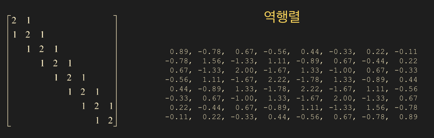
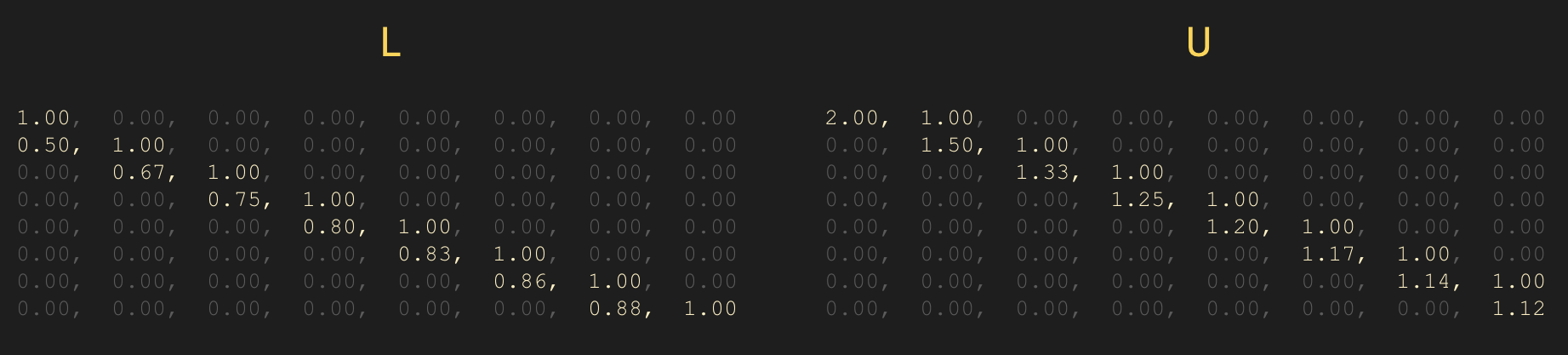
• In summary, unless you specifically need the inverse matrix $A^{-1}$, do not calculate the inverse when solving $A\mathbf{x} = \mathbf{b}$!

Calculating the Inverse

• If your goal for finding the inverse is to solve $A\mathbf{x} = \mathbf{b}$, you should reconsider.
• Use linalg.inv(matrix) to find the inverse matrix.

• If the input matrix is not invertible (i.e., it is a singular matrix), an error will occur.

• The basic algorithm uses LU decomposition and solves $\quad LUA^{-1} = I$, going through only the backward phase (back substitution).

A1 = np.array([[1,2,1],[2,1,3],[1,3,1]])
inv_a1 = linalg.inv(A1)

prt(inv_a1, fmt="%0.2f")

 8.00, -1.00, -5.00
-1.00,  0.00,  1.00
-5.00,  1.00,  3.00

Solving the Matrix Equation Ax = b

• Solving $A\mathbf{x} = \mathbf{b}$ is equivalent to finding $\mathbf{x}$.

• You can use the x = linalg.solve(A, b, assume_a="gen") function.
• The assume_a parameter accepts four types of inputs.

gen
General solver. Used when the matrix type (symmetric, hermitian, etc.) is unknown.
Solves via LU decomposition: $\quad A = LU$

sym
Used for symmetric or complex symmetric matrices. Note that complex symmetric is not the same as Hermitian.
A symmetric matrix satisfies $\; A = A^T \;$.
Uses diagonal pivoting: $\quad A = LDL^T \mbox{(block diagonal)}$.

her
Used for Hermitian matrices: $\quad A = A^$ (conjugate transpose).
Solves via diagonal pivoting: $\quad A = LDL^$.

pos
Used for positive definite matrices. Implies the quadratic form $\mathbf{x}^TA\mathbf{x} > 0$. Uses Cholesky Decomposition: $\quad A = R^TR = LL^T$

• Be careful, as setting assume_a incorrectly may not trigger an error but will return wrong results. Therefore, gen is commonly used.
• If you understand the matrix properties well, using the assume_a option is beneficial for computation speed.

b = np.ones((3,), dtype=np.float64)

# singular (not invertible)
A_sing = np.array([[1,3,4],[-4,2,-6],[-3,-2,-7]])

# gen (general)
A_gen = np.array([[0,1,2],[1,0,3],[4,-3,8]])

# sym (symmetric)
A_sym = np.array([[1,2,1],[2,1,3],[1,3,1]])

# sym complex (symmetric complex)
A_sym_c = np.array([[1, 2-1j, 1+2j],[2-1j, 1, 3],[1+2j, 3,1]])

# her (hermitian)
A_her = np.array([[1, 2+1j, 1-2j],[2-1j, 1, 3],[1+2j, 3,1]])

# pos (positive definite)
A_pos = np.array([[2, -1, 0],[-1,2,-1],[0,-1,2]])

• singular
• An error occurs because it is a singular matrix.

x = linalg.solve(A_sing, b) 

numpy.linalg.LinAlgError: Matrix is singular.

• gen
• Added the last line to determine if $Ax = b ightarrow Ax - b = 0$.

x = linalg.solve(A_gen, b)

prt(x, fmt="%0.5e")
print()
prt(A_gen @ x - b , fmt="%0.5e")

 1.00000e+00,  1.00000e+00,  0.00000e+00

 0.00000e+00,  0.00000e+00,  0.00000e+00

• sym
• The difference between sym and gen lies in the underlying algorithm.
• Keep in mind that the solution x we obtain is an approximation. Errors occur in values calculated using LU decomposition (gen) versus diagonal pivoting (sym).

x1 = linalg.solve(A_sym, b) # default is gen
x2 = linalg.solve(A_sym, b, assume_a="sym")

prt(x1, fmt="%0.5e")
print()
prt(A_sym @ x1 - b , fmt="%0.5e")

prt(x2, fmt="%0.5e")
print()
prt(A_sym @ x2 - b , fmt="%0.5e")

 # gen
 2.00000e+00,  0.00000e+00, -1.00000e+00

 0.00000e+00,  0.00000e+00,  0.00000e+00

# sym
 2.00000e+00, -2.77556e-17, -1.00000e+00

 0.00000e+00,  0.00000e+00,  0.00000e+00

• her

x = linalg.solve(A_her, b, assume_a="her")

prt(x, fmt="%0.5e")
print()
prt(A_her @ x - b , fmt="%0.5e")

( 1.11111e-01+1.11111e-01j), ( 3.33333e-01-1.11111e-01j), ( 1.11111e-01+1.11022e-16j)

( 0.00000e+00+2.77556e-17j), (-4.44089e-16+1.94289e-16j), ( 2.22045e-16-1.66533e-16j)

• Here, e-16 means $10^{-16}$, which is close to 0.

• pos

x1 = linalg.solve(A_pos, b, assume_a="gen")
x2 = linalg.solve(A_pos, b, assume_a="pos")

prt(x1, fmt="%0.5e")
print()
prt(A_pos @ x1 - b , fmt="%0.5e")

prt(x2, fmt="%0.5e")
print()
prt(A_pos @ x2 - b , fmt="%0.5e")

# gen
 1.50000e+00,  2.00000e+00,  1.50000e+00

 0.00000e+00,  2.22045e-16, -4.44089e-16

# pos
 1.50000e+00,  2.00000e+00,  1.50000e+00

-8.88178e-16,  1.55431e-15, -4.44089e-16

Triangular Matrix Solver

• This also solves $A\mathbf{x} = \mathbf{b}$, but only when matrix $A$ is a lower triangular or upper triangular matrix.
• Only the backward phase (back substitution) is required.
• x = linalg.solve_triangular(A, b, lower=False)
• Set the lower parameter to True for lower triangular and False for upper triangular.

A = np.array([[1,0,0,0],[1,4,0,0],[5,0,1,0],[8,1,-2,2]], dtype=np.float64)
b = np.array([1,2,3,4],dtype=np.float64)

x = linalg.solve_triangular(A, b, lower=True)

prt(x, fmt="%0.5e")

 1.00000e+00,  2.50000e-01, -2.00000e+00, -4.12500e+00

Is the Solution Accurate?

• The solution x we obtain when solving $A\mathbf{x} = \mathbf{b}$ is an approximation resulting from numerical calculations.

• Is $A\mathbf{x}$ similar enough to $\mathbf{b}$? This is equivalent to asking if $A\mathbf{x} - \mathbf{b}$ is close enough to 0.

• You can compare $A\mathbf{x} - \mathbf{b}$ with a zero matrix created via np.zeros using the np.allclose function.

A = np.array([[2,-1,0],[-1,2,-1],[0,-1,2]], dtype=np.float64)
b = np.ones((3,), dtype=np.float64)

x = linalg.solve(A, b, assume_a="pos")

prt(x, fmt="%0.5e")
print()
prt(A@x-b, fmt="%0.5e")

zr = np.zeros((3,), dtype=np.float64)

bool_close = np.allclose(A@x-b, zr)
print(bool_close)

 1.50000e+00,  2.00000e+00,  1.50000e+00

-8.88178e-16,  1.55431e-15, -4.44089e-16
True

Example 1.

$A = \begin{bmatrix} 1 & 1/2 & 1/3 & \dots & 1/9 & 1/10 \ 1/2 & 1/3 & 1/4 & \dots & 1/10 & 1/11 \ 1/3 & 1/4 & 1/5 & \dots & 1/11 & 1/12 \ \vdots & \ddots & \ddots & & & \ 1/9 & 1/10 & & & 1/17 & 1/18 \ 1/10 & 1/11 & \dots & \dots & 1/18 & 1/19 \end{bmatrix} $

Create a 10x10 Hilbert matrix using linalg.hilbert(10) and store it in A.
Store the inverse of A in inv_A.
Calculate x1 = inv_A @ b.
Calculate x2 using linalg.solve (gen).
Print A@x1 - b with 15 decimal places using custom output (floating).
Print A@x2 - b with 15 decimal places using custom output (floating).
Compare A@x1 - b and A@x2 - b with a zero vector using allclose.

• Solution
• The Hilbert matrix is numerically very difficult to handle. As its size increases, it becomes harder to solve accurately.
• Although we learned the theory, we can see that solving via inverse matrix is inferior in terms of accuracy.

A = linalg.hilbert(10)
b = np.ones((10,), dtype=np.float64)

# Hilbert Matrix
prt(A, fmt="%0.5f")

A_inv = linalg.inv(A)

x1 = A_inv @ b

print()

x2 = linalg.solve(A, b, assume_a="gen")

prt(A @ x1 - b, fmt="%0.15e")
print()
prt(A @ x2 - b, fmt="%0.15e")
print()

zr = np.zeros((10,), dtype=np.float64)

bool_close1 = np.allclose(A @ x1 - b, zr)
print(bool_close1)

bool_close2 = np.allclose(A @ x2 - b, zr)
print(bool_close2)

• Output of the Hilbert Matrix:

  1.00000,  0.50000,  0.33333,  0.25000,  0.20000,  0.16667,  0.14286,  0.12500,  0.11111,  0.10000
   0.50000,  0.33333,  0.25000,  0.20000,  0.16667,  0.14286,  0.12500,  0.11111,  0.10000,  0.09091
   0.33333,  0.25000,  0.20000,  0.16667,  0.14286,  0.12500,  0.11111,  0.10000,  0.09091,  0.08333
   0.25000,  0.20000,  0.16667,  0.14286,  0.12500,  0.11111,  0.10000,  0.09091,  0.08333,  0.07692
   0.20000,  0.16667,  0.14286,  0.12500,  0.11111,  0.10000,  0.09091,  0.08333,  0.07692,  0.07143
   0.16667,  0.14286,  0.12500,  0.11111,  0.10000,  0.09091,  0.08333,  0.07692,  0.07143,  0.06667
   0.14286,  0.12500,  0.11111,  0.10000,  0.09091,  0.08333,  0.07692,  0.07143,  0.06667,  0.06250
   0.12500,  0.11111,  0.10000,  0.09091,  0.08333,  0.07692,  0.07143,  0.06667,  0.06250,  0.05882
   0.11111,  0.10000,  0.09091,  0.08333,  0.07692,  0.07143,  0.06667,  0.06250,  0.05882,  0.05556
   0.10000,  0.09091,  0.08333,  0.07692,  0.07143,  0.06667,  0.06250,  0.05882,  0.05556,  0.05263
  

• Comparison of results from inverse matrix vs np.solve (gen):

-5.384686879750245e-05, -4.824035864248177e-05, -4.365437722742005e-05, -3.984553430069759e-05, -3.663714443313815e-05, -3.390060580654719e-05, -3.154054138576612e-05, -2.948524204493541e-05, -2.767985240692550e-05, -2.608172012175114e-05

 1.768403201651836e-10,  2.589735093039280e-10,  1.027888885118955e-11, -5.332401187274627e-13, -2.094682205466825e-10, -1.216354794664198e-10,  8.731149137020111e-11,  4.546962806273314e-11,  5.050826423769195e-11, -6.052347512053302e-11

False
True