Numpy & Scipy - 1.5 Basic Manipulation of Matrices (3)

Addition and Subtraction of Matrices and Vectors of the Same Size

$A = \begin{bmatrix} 1 & 2 \ 3 & 4 \end{bmatrix}$ $B = \begin{bmatrix} 5 & 6 \ 7 & 8 \end{bmatrix}$

A = np.array([[1,2], [3,4]])

B = np.array([[5,6],[7,8]])

C = A + B

C = A - B

• Vectors (1D arrays) can also be added and subtracted in the same way.
• As long as the shape is exactly the same, there are no problems.

Easily Creating Large Matrices

$ A = \begin{bmatrix} 2 & 1 & 0 & 0 & 0 \ -1 & 2 & 1 & 0 & 0 \ 0 & -1 & 2 & 1 & 0 \ 0 & 0 & -1 & 2 & 1 \ 0 & 0 & 0 & -1 & 2 \end{bmatrix} = \begin{bmatrix} 0 & 0 & 0 & 0 & 0 \ -1 & 0 & 0 & 0 & 0 \ 0 & -1 & 0 & 0 & 0 \ 0 & 0 & -1 & 0 & 0 \ 0 & 0 & 0 & -1 & 0 \end{bmatrix} + \begin{bmatrix} 2 & 0 & 0 & 0 & 0 \ 0 & 2 & 0 & 0 & 0 \ 0 & 0 & 2 & 0 & 0 \ 0 & 0 & 0 & 2 & 0 \ 0 & 0 & 0 & 0 & 2 \end{bmatrix} + \begin{bmatrix} 0 & 1 & 0 & 0 & 0 \ 0 & 0 & 1 & 0 & 0 \ 0 & 0 & 0 & 1 & 0 \ 0 & 0 & 0 & 0 & 1 \ 0 & 0 & 0 & 0 & 0 \end{bmatrix} $

• Here, extract each band into a 1D array using np.ones and multiply by a scalar value.

For $k = -1$
$ b_1 = \begin{bmatrix} -1 & -1 & -1 & -1 \end{bmatrix} $

b1 = (-1)*np.ones((4,))

For $k = 0$
$ b_2 = \begin{bmatrix} 2 & 2 & 2 & 2 & 2 \end{bmatrix} $

b2 = (2)*np.ones((5,))

For $k = 1$
$ b_3 = \begin{bmatrix} 1 & 1 & 1 & 1 \end{bmatrix} $

b3 = (1)*np.ones((4,))

• Then use the np.diag function to turn these 1D arrays into matrices based on the maximum size (k=0) and add them together.

A = np.diag(b1, k=-1) + np.diag(b2, k=0) + np.diag(b3, k=1)

print(A)

[[ 2.  1.  0.  0.  0.]
 [-1.  2.  1.  0.  0.]
 [ 0. -1.  2.  1.  0.]
 [ 0.  0. -1.  2.  1.]
 [ 0.  0.  0. -1.  2.]]

Addition of Scalar and Matrix (r + A)

• Mathematically it doesn’t make sense, but it is possible in Python…
• It adds the scalar to every entry. Same goes for vectors.

A = np.array([[1,2],[3,4]])

r = 5

result = r + A # = A + r

print(result)

[[6 7]
 [8 9]]

Element-wise Multiplication and Division of Matrices (A * B) (A / B)

• Be careful, this is NOT matrix multiplication. It is completely different from A @ B or np.matmul!!
• Matrices with the same shape can be multiplied.
• It multiplies the entries at the same index and returns the result. Same for vectors.

A = np.array([[1,2],[3,4]])
B = np.array([[5,6],[7,8]])

result = A * B # = B * A

print(result)

[[ 5 12]
 [21 32]]

• Division works the same way.
• It doesn’t mean inverse matrix, it’s just simple element-wise division.

A = np.array([[1,2],[3,4]])
B = np.array([[5,6],[7,8]])

result = A / B # = B / A

print(result)

[[0.2        0.33333333]
 [0.42857143 0.5       ]]

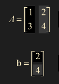
Element-wise Multiplication and Division of Matrix and Vector (A * b) (A / b)

• Be careful, this is NOT matrix-vector product.
• The shapes are different, but it’s possible…
• The number of columns in the matrix must equal the size of the vector. (A.shape[1] == b.shape[0])
• For division, A / b and b / A give different results because the operation method itself is different.

• Multiplication/division occurs between areas of the same color in the image above.

A = np.array([[1,2],[3,4]])
b = np.array([2,4])

result = A * b

print(result)

result = A / b

print(result)

result = b / A # Think of it as b * (1 / A)

print(result)

[[ 2  8]
 [ 6 16]]

 [[0.5 0.5]
 [1.5 1. ]]

[[2.         2.        ]
 [0.66666667 1.        ]]

Reconstructing Part of a Matrix Using Index Arrays

A = np.array([[1,2,3,4,5],[6,7,8,9,10],[11,12,13,14,15],[-1,-2,-3,-4,-5]])

print(A)

what_i_want = A[[1,2,0,3], : ]

# or

idx = [1,2,0,3]
what_i_want = A[idx, :]

print(what_i_want)

# matrix A
[[ 1  2  3  4  5]
 [ 6  7  8  9 10]
 [11 12 13 14 15]
 [-1 -2 -3 -4 -5]]

# index array
[[ 6  7  8  9 10]
 [11 12 13 14 15]
 [ 1  2  3  4  5]
 [-1 -2 -3 -4 -5]]

• Extracting only rows

idx = [2,1]

what_i_want = A[idx, :]

print(what_i_want)

[[11 12 13 14 15]
 [ 6  7  8  9 10]]

• Extracting columns is also possible

idx = [4,1,2]

what_i_want = A[:, idx]

print(what_i_want)

[[ 5  2  3]
 [10  7  8]
 [15 12 13]
 [-5 -2 -3]]

• Combining both

idx_r = [2,3,0] # row
idx_c = [2,1,3] # column

what_i_want = A[idx_r, :][:, idx_c] # =  A[:, idx_c][idx_r, :]

print(what_i_want)

[[13 12 14]
 [-3 -2 -4]
 [ 3  2  4]]