Numpy & Scipy - 1.4 Basic Manipulation of Matrices (2)

hstack / vstack

• np.hstack((tuple)), np.vstack((tuple)): Allows combining 2D arrays, 1D arrays, or a mix of both.
• Both perform deep copies.

• (1) Case of 2D array

• 2x3 2x2 hstack

a = np.array([[1,2,3], [4,5,6]], dtype=np.float64)
b = np.array([[-1,-2], [-3,-4]], dtype=np.float64) 

new_mat = np.hstack( (a,b) ) # Note that input is a tuple

new_mat = np.hstack( (a,b,b,b) ) # Multiple combinations possible

prt(new_mat, fmt="%0.1f", delimiter=",")
print()
print(new_mat.shape)

# You can see the matrices are combined horizontally.
1.0, 2.0, 3.0,-1.0,-2.0
4.0, 5.0, 6.0,-3.0,-4.0

# 2x5 matrix
(2, 5)

• 3x3 2x2 hstack

a = np.array([[1,2,3],[4,5,6]], dtype=np.float64)
b = np.array([[-1,-2,-3],[-4,-5,-6],[-7,-8,-9]], dtype=np.float64)

new_mat = np.hstack( (a,b) ) # Note input is tuple

prt(new_mat, fmt="%0.1f", delimiter=",")
print()
print(new_mat.shape)

# 2x3 and 3x3 cannot be hstacked (2 rows vs 3 rows)
ValueError: all the input array dimensions except for the concatenation axis must match exactly, but along dimension 0, the array at index 0 has size 2 and the array at index 1 has size 3

• 2x3 2x2 vstack

a = np.array([[1,2,3], [4,5,6]], dtype=np.float64)
b = np.array([[-1,-2], [-3,-4]], dtype=np.float64) 

new_mat = np.vstack( (a,b) ) # Note input is tuple

prt(new_mat, fmt="%0.1f", delimiter=",")
print()
print(new_mat.shape)

# 2x3 and 2x2 cannot be vstacked, causing the following error.

ValueError: all the input array dimensions except for the concatenation axis must match exactly, but along dimension 1, the array at index 0 has size 3 and the array at index 1 has size 2

• 2x3 3x3 vstack

a = np.array([[1,2,3],[4,5,6]], dtype=np.float64)
b = np.array([[-1,-2,-3],[-4,-5,-6],[-7,-8,-9]], dtype=np.float64)

new_mat = np.vstack( (a,b) ) # Note input is tuple

prt(new_mat, fmt="%0.1f", delimiter=",")
print()
print(new_mat.shape)

1.0, 2.0, 3.0
4.0, 5.0, 6.0
-1.0,-2.0,-3.0
-4.0,-5.0,-6.0
-7.0,-8.0,-9.0

(5, 3)

(2) Case of 1D array

• hstack
• The 1D array vector becomes longer.

a = np.array([1,2,3], dtype=np.float64)
b = np.array([4,5,6], dtype=np.float64)

new_mat = np.hstack( (a,b) ) # Note input is tuple

prt(new_mat, fmt="%0.1f", delimiter=",")
print()
print(new_mat.shape)

1.0, 2.0, 3.0, 4.0, 5.0, 6.0

(6,)

• vstack
• A matrix is created.

a = np.array([1,2,3], dtype=np.float64)
b = np.array([4,5,6], dtype=np.float64)

new_mat = np.vstack( (a,b) ) # Note input is tuple

prt(new_mat, fmt="%0.1f", delimiter=",")
print()
print(new_mat.shape)

1.0, 2.0, 3.0
4.0, 5.0, 6.0

(2, 3)

• (3) Mixed 2D array and 1D array

• hstack
• hstack will always error. Mixed types work only with vstack.

a = np.array([[1,2,3],[4,5,6]],dtype=np.float64)
b = np.array([7,8,9], dtype=np.float64)

new_mat = np.hstack( (a,b) ) # Note input is tuple

prt(new_mat, fmt="%0.1f", delimiter=",")
print()
print(new_mat.shape)

ValueError: all the input arrays must have same number of dimensions, but the array at index 0 has 2 dimension(s) and the array at index 1 has 1 dimension(s)

• vstack
• Combining 2x3 2D array and 1x3 1D array

a = np.array([[1,2,3],[4,5,6]],dtype=np.float64)
b = np.array([7,8,9], dtype=np.float64)

new_mat = np.vstack( (a,b) ) # Note input is tuple

prt(new_mat, fmt="%0.1f", delimiter=",")
print()
print(new_mat.shape)

1.0, 2.0, 3.0
4.0, 5.0, 6.0
7.0, 8.0, 9.0

(3, 3)

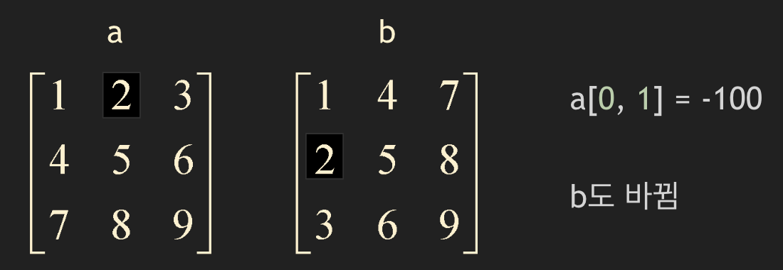
transpose method

• Literally transposes the matrix.

• It is a shallow copy.

• (1) transpose property

c = np.array([[1,2,3],[4,5,6],[7,8,9]], dtype=np.float64)

d = c.T

prt(c, fmt="%0.1f", delimiter=",")
print()
prt(d, fmt="%0.1f", delimiter=",")

# c matrix
1.0, 2.0, 3.0
4.0, 5.0, 6.0
7.0, 8.0, 9.0

# d matrix (transpose of c)
1.0, 4.0, 7.0
2.0, 5.0, 8.0
3.0, 6.0, 9.0

• shallow copy example

• (2) transpose method

• If you transpose() a 1D array, it remains a 1D array.

e = np.array([1,2,3], dtype=np.float64)

f = e.transpose()

g = np.copy(e.transpose()) # deep copy is possible via np.copy

prt(e, fmt="%0.1f", delimiter=",")
print(e.shape)
print()
prt(f, fmt="%0.1f", delimiter=",")
print(f.shape)

1.0, 2.0, 3.0
(3,)

1.0, 2.0, 3.0
(3,)

real / imag / conjugate

• real, imag return the real and imaginary parts of each matrix entry respectively.
• imag takes the imaginary part and returns it as a real matrix or vector.

• Both are shallow copies.

• conjugate is a deep copy.

a = np.array([[1-2j, 3+1j, 1], [1+2j, 2-1j, 7]], dtype=np.complex128)

a_real = r.real

# prt(a, fmt="%0.1f", delimiter=",")
# print()
# prt(a_real, fmt="%0.1f", delimiter=",")

a_imag = r.imag # Returns imaginary part as real numbers

# prt(a, fmt="%0.1f", delimiter=",")
# print()
# prt(a_imag, fmt="%0.1f", delimiter=",")


a_conj = r.conjugate() # conjugate multiplies imaginary part by -1
# deep copy

# prt(a, fmt="%0.1f", delimiter=",")
# print()
# prt(a_conj, fmt="%0.1f", delimiter=","

# a matrix
( 1.0-2.0j),( 3.0+1.0j),( 1.0+0.0j)
( 1.0+2.0j),( 2.0-1.0j),( 7.0+0.0j)

# real
1.0, 3.0, 1.0
1.0, 2.0, 7.0

# imag
-2.0, 1.0, 0.0
 2.0,-1.0, 0.0

# conjugate
( 1.0+2.0j),( 3.0-1.0j),( 1.0+0.0j)
( 1.0-2.0j),( 2.0+1.0j),( 7.0+0.0j)

Multiplication

• Scalar Multiplication
• Order does not matter: result = r * A = A * r

A = np.array([[1,2,1],[2,1,3],[1,3,1]], dtype=np.float64)
scalar = 5.0

result = scalar * A

prt(A, fmt="%0.1f", delimiter=",")
print()
prt(result, fmt="%0.1f", delimiter=",")

1.0, 2.0, 1.0
2.0, 1.0, 3.0
1.0, 3.0, 1.0

5.0, 10.0, 5.0
10.0, 5.0, 15.0
5.0, 15.0, 5.0

• Matrix Multiplication

• Order is very important. Same as mathematical matrix multiplication.

• Can use @ operator or np.matmul() function.

A = np.array([[1,2,3], [3,2,1]], dtype=np.float64)
B = np.array([[2,1],[1,2],[-3, 3]], dtype=np.float64)

result = A @ B
result2 = np.matmul(A, B)

prt(A, fmt="%0.1f", delimiter=",")
print()
prt(B, fmt="%0.1f", delimiter=",")
print()
prt(result, fmt="%0.1f", delimiter=",")
print()
prt(result2, fmt="%0.1f", delimiter=",")

1.0, 2.0, 3.0
3.0, 2.0, 1.0

2.0, 1.0
1.0, 2.0
-3.0, 3.0

# A @ B
-5.0, 14.0
 5.0, 10.0

# np.matmul(A,B)
-5.0, 14.0
 5.0, 10.0

• Matrix-Vector Multiplication
• Similarly, calculated using result = A @ u or result = np.matmul(A,u).
• NOT dot product!

A = np.array([[1,2,1],[2,1,3],[1,3,1]], dtype=np.float64)
u = np.array([5,1,3], dtype=np.float64)

Au = np.matmul(A, u)

prt(A, fmt="%0.1f", delimiter=",")
print()
prt(u, fmt="%0.1f", delimiter=",")
print()
prt(Au, fmt="%0.1f", delimiter=",")

1.0, 2.0, 1.0
2.0, 1.0, 3.0
1.0, 3.0, 1.0

5.0, 1.0, 3.0

10.0, 20.0, 11.0

Inner Product : vdot

• result = np.vdot(u, v)

• Here u, v are vectors.

• Inner Product is expressed as a linear combination:

real vector : $\quad \mathbf{u} \cdot \mathbf{v} = u_1v_1 + u_2v_2 + \dots + u_nv_n$
complex vector : $ \quad \mathbf{u} \cdot \mathbf{v} = u_1\bar{v}_1 + u_2\bar{v}_2 + \dots + u_n\bar{v}_n = \bar{u_1v_1} + \bar{u_2v_2} + \dots + \bar{u_nv_n}$

• Example..

u = np.array([1,1,1,1], dtype=np.float64)
v = np.array([-1,1,-1,1], dtype=np.float64)

vdot = np.vdot(u,v)

prt(u, fmt="%0.1f", delimiter=",")
print()
prt(v, fmt="%0.1f", delimiter=",")
print()
print(vdot)

 1.0, 1.0, 1.0, 1.0

-1.0, 1.0,-1.0, 1.0

0.0

Norm

• The vector norm we learned in linear algebra is defined as \(\lVert \mathbf{x} Vert _2 = \left( \sum_{i=1}^n x_i^2 ight)^{1/2} \quad l_2 \mbox{-vector norm (Euclidean)}\), which is called the $l_2$ norm. There are many other vector norms.

vector norm

\[\lVert \mathbf{x} Vert _1 = \sum_{i=1}^n \lvert x_i vert \quad l_1 \mbox{-vector norm}\] \[\lVert \mathbf{x} Vert _2 = (\sum_{i=1}^n \lvert x_i^2 vert)^{1/2} \quad l_2 \mbox{-vector norm (Euclidean)}\] \[\lVert \mathbf{x} Vert _{\infty} = \max_{1 \le i \le n} \lvert x_i vert\]

• Similarly, matrix norms exist, like $l_1, l_2, l_{\infty}$ norms for vectors.

matrix norm

\[\lVert A Vert _1 = \max_{1 \le j \le n} \sum_{i=1}^m \lvert a_{ij} vert \quad l_1 \mbox{-matrix norm}\] \[\lVert A Vert _2 = \sigma _{\max} \le \left( \sum_{i=1}^m \sum_{j=1}^n \lvert a_{ij} vert ^2 ight)^{1/2} \quad l_2 \mbox{-matrix norm (spectral)}\] \[\lVert A Vert _{\infty} = \max_{1 \le i \le m} \sum_{j=1}^n \lvert a_{ij} vert \quad l_{\infty} \mbox{-matrix norm}\]

• To calculate using linalg.norm in numpy, you need the scipy library.

from scipy import linalg

• Example

w = np.array([1,1], dtype=np.float64)

norm = linalg.norm(w, 2)

prt(w, fmt="%0.1f", delimiter=",")
print()
print(norm)

 1.0, 1.0

 1.4142135623730951

• To find $l_{\infty}$ norm, pass inf as a parameter.

norm = linalg.norm(a, 2, inf)

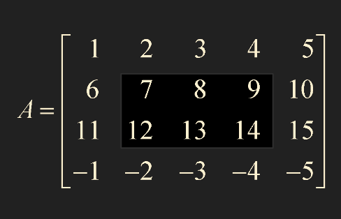
slicing - Extracting part of a matrix or vector

• It is a shallow copy.

• Example

A = np.array([[1,2,3,4,5], [6,7,8,9,10], [11,12,13,14,15], [-1,-2,-3,-4,-5]])
sub_A = A[1:3, 1:4]

• row: 1~2, column: 1~3.
• i.e., up to index -1 of the number after :.
• 1:3 actually gets up to 1:2.

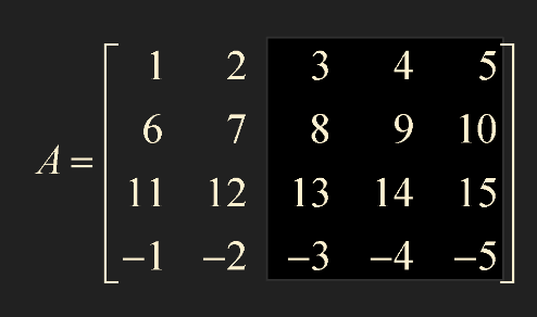
sub_A = A[0:5, 2:6]

# Same as below

sub_A = A[ : , 2: ]

• : means from start to end.
• 2: means from 2 to the end.

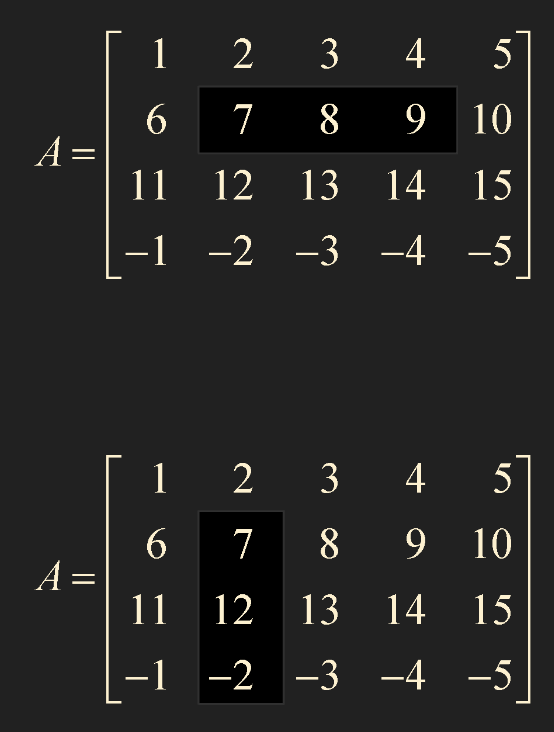
• If slicing operator : is not attached to row or column side, it returns a 1D array.
• Can convert to 2D array via np.reshape.

sub_A1 = A[1:2, 1:4] # Returns as 2D array
sub_A2 = A[1, 1:4] # Returns as 1D array

sub_A3 = A[1: , 1:2] # Returns as 2D array
sub_A4 = A[1:, 1] # Returns as 1D array

sub_A5 = np.reshape(sub_A3, (3,1)) # 1D array -> 2D array

#sub_A1
7.0, 8.0, 9.0
(1, 3)

#sub_A2
7.0, 8.0, 9.0
(3,)

#sub_A3
 7.0
 12.0
-2.0
(3, 1)

#sub_A4
7.0, 12.0,-2.0
(3,)

#sub_A5
 7.0
 12.0
-2.0
(3, 1)

Example 1.

$A = \begin{bmatrix} 1 & 2 \ 3 & 4 \end{bmatrix} \quad \mathbf{x} = \begin{bmatrix} 5 \ 6 \end{bmatrix} $
Store $A, \mathbf{x}$ in variables as 2D and 1D arrays respectively. Given that 1D array cannot be transposed, calculate the quadratic form $\mathbf{x}^TA\mathbf{x}$.
1) Try converting to 2D array (np.reshape)
2) Try using np.vdot

import numpy as np
from print_lecture import print_custom as prt
from scipy import linalg

A = np.array([[1,2],[3,4]], dtype=np.float64)
x = np.array([5,6], dtype=np.float64)

# 1) 
x_t = np.reshape(x, (2,1))

result1 = np.matmul(np.matmul(x_t.T, A), x)

print(result1)

# 2) np.vdot 

result2 = np.vdot(x, A @ x)

print(result2)

# Result 1
319.0

# Result 2
319.0