Flow Field Pathfinding - The Optimal Solution for Massive Crowds

Introduction

Imagine 3,000 zombies swarming toward the player. If you compute an individual path for each zombie? A single A* search traverses hundreds to thousands of nodes, and you’d have to repeat that 3,000 times. Framerate tanks instantly.

Flow Field pathfinding approaches this problem in a fundamentally different way. Instead of giving each agent a path, it inscribes “where to go” across the entire space. An agent simply reads the direction at the spot where it stands.

This post covers the core concepts of Flow Field and its 3-stage pipeline, and analyzes why it is practically the only viable option for large-scale crowd simulation.

The video below shows an early implementation where 3,000 agents track the player in real time via Flow Field. The entire pipeline is parallelized with Unity Jobs + Burst.

---

Part 1: The Limits of Traditional Pathfinding

A* Algorithm — Fast, but Doesn’t Scale

A* is the de facto standard for game pathfinding. It leverages heuristics to find the shortest path faster than Dijkstra and is a perfect solution for a handful of agents.

But the story changes as agent count grows.

Cost When You Have N Agents

A*’s time complexity depends on grid size and path length. In general, it’s \(O(E \log V)\) where \(E\) is the number of explored edges and \(V\) is the number of nodes. The problem is that this must be repeated for every agent.

Agent Count	A* Total Cost	Flow Field Total Cost
1	\(O(E \log V)\)	\(O(V)\)
10	\(O(10 \cdot E \log V)\)	\(O(V)\)
100	\(O(100 \cdot E \log V)\)	\(O(V)\)
3,000	\(O(3000 \cdot E \log V)\)	\(O(V)\)

Flow Field computes the entire grid only once, regardless of agent count. The more agents you have, the more dramatic the advantage over A* becomes.

Additional Issues with A*

• Redundant paths: Agents heading for the same destination recompute nearly identical paths
• Dynamic obstacles: Every agent’s path must be recomputed whenever the environment changes
• Memory: Each agent must store its own path list (waypoint array)
• Crowd flow: Individual paths don’t produce natural crowd flow (overlapping at bottlenecks)

---

Part 2: The Core Idea Behind Flow Field

Computing a “Field,” Not a “Path”

While A* finds a path from start to goal, Flow Field computes a direction from every point to the goal.

An analogy:

A* is like a GPS navigator — you have to search for a route from each starting point. Flow Field is like terrain where water flows — no matter where you drop water, it naturally flows downhill to the lowest point.

Once the Flow Field is complete, each agent’s movement becomes trivial:

1. Determine which cell I'm in
2. Read the direction vector of that cell
3. Move in that direction

The lookup cost per agent is \(O(1)\). Whether it’s 3,000 or 10,000 agents makes no difference.

The 3-Stage Pipeline

Flow Field computes three independent fields sequentially:

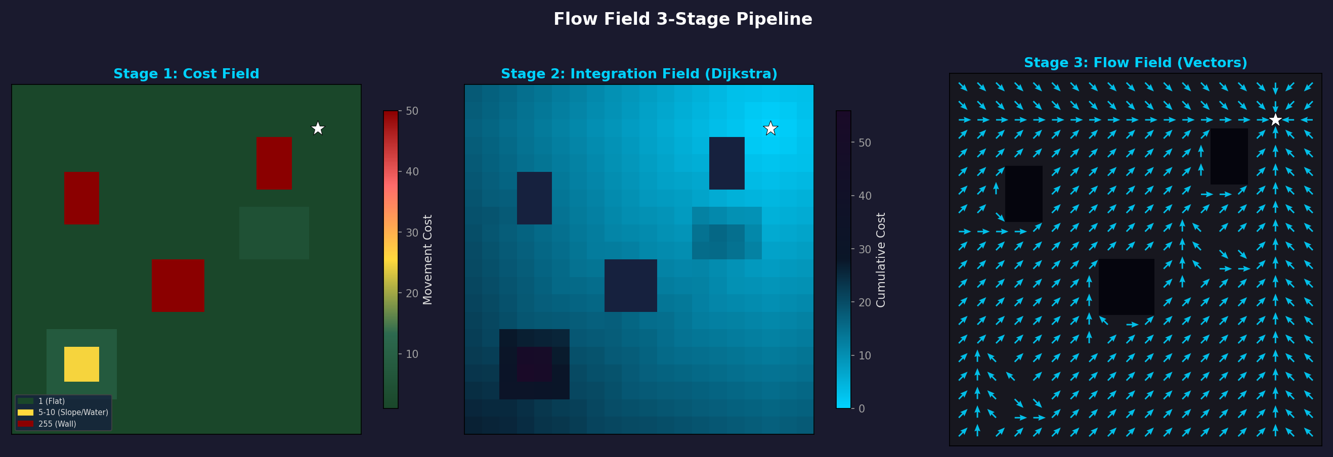Cost Field → Integration Field (Dijkstra) → Flow Field (direction vectors). A natural detour around obstacles (black squares) emerges.

flowchart LR
    A["<b>Cost Field</b><br/>Movement cost per cell<br/>(terrain, obstacles)"] --> B["<b>Integration Field</b><br/>Cumulative cost<br/>to destination"] --> C["<b>Flow Field</b><br/>Movement direction<br/>vector per cell"]
    
    style A fill:#e8d5b7,stroke:#b8860b,color:#333
    style B fill:#b7d5e8,stroke:#4682b4,color:#333
    style C fill:#b7e8c4,stroke:#2e8b57,color:#333

Because each stage is independent:

• Cost Field is only recomputed when terrain changes (barricade placed/destroyed)
• Integration Field is only recomputed when the destination moves
• Flow Field is only recomputed when the Integration Field changes

This caching strategy is what makes Flow Field practical for real-time games.

---

Part 3: Cost Field — Representing the World as a Grid

Grid Structure

The Cost Field is a 2D grid that divides the game world into uniform square cells.

Parameter	Description	Typical Values
Cell Size	Length of one cell edge	0.5 – 2.0 units
Grid Width × Height	Grid dimensions	200×200 – 500×500
Data Type	Storage per cell	byte (0–255)

Cell size is a tradeoff between precision and performance:

• Small cells (0.5): Precise obstacle representation, but 4× the computation
• Large cells (2.0): Fast computation, but may fail to represent narrow passages

What the Cost Values Mean

The cost assigned to each cell represents “how difficult is it to traverse this cell.”

Cost	Meaning	Example
1	Flat ground	Roads, level terrain
2–4	Rough terrain	Mud, shallow water, gentle slopes
5–10	High-cost terrain	Steep slopes, deep water
255	Impassable	Walls, buildings, cliffs

Slope-Based Cost Calculation

In actual 3D terrain, height differences must be reflected in the cost. The slope is calculated from the height difference \(\Delta h\) between adjacent cells:

\[\text{slope} = \frac{\Delta h}{\text{cellSize}}\]

This slope is then converted to a cost based on thresholds:

Slope Range	Classification	Additional Cost
0 – 0.3	Gentle	+0
0.3 – 0.6	Moderate	+3
0.6 – 1.0	Steep	+8
Above 1.0	Impassable	255

This produces the natural behavior of agents detouring around steep hills.

Dynamic Cost Updates

The environment can change during gameplay:

• Barricade placed → Set the cell to 255 (impassable)
• Barricade destroyed → Restore original cost
• Bridge built → Set water cells’ cost to 1

Dynamic updates to the Cost Field only need to modify the changed cells, so the cost is very low. However, when the Cost Field changes, the Integration Field and Flow Field must be recomputed.

---

Part 4: Integration Field — Cumulative Cost to the Destination

Concept

The Integration Field is the result of computing “the total cost to travel from this cell to the destination” for every cell in the grid.

The computation method is a variant of Dijkstra’s algorithm. Starting from the destination cell, costs propagate outward to neighboring cells:

1. Destination cell cumulative cost = 0
2. Destination's neighbors = neighbor's cost value
3. Neighbor's neighbors = previous cumulative cost + that cell's cost value
4. Repeat until all reachable cells are filled

Example: 5×5 Grid

With the destination at center (2,2) and all cells having a cost of 1:

┌─────┬─────┬─────┬─────┬─────┐
│  4  │  3  │  2  │  3  │  4  │   Integration
│     │     │     │     │     │   Field
├─────┼─────┼─────┼─────┼─────┤
│  3  │  2  │  1  │  2  │  3  │   (Cumulative cost
│     │     │     │     │     │    from destination)
├─────┼─────┼─────┼─────┼─────┤
│  2  │  1  │  0  │  1  │  2  │   0 = Destination
│     │     │     │     │     │
├─────┼─────┼─────┼─────┼─────┤
│  3  │  2  │  1  │  2  │  3  │
│     │     │     │     │     │
├─────┼─────┼─────┼─────┼─────┤
│  4  │  3  │  2  │  3  │  4  │
│     │     │     │     │     │
└─────┴─────┴─────┴─────┴─────┘

When obstacles are present, the cumulative cost reflects routes that detour around them:

┌─────┬─────┬─────┬─────┬─────┐
│  6  │  5  │  4  │  3  │  4  │
│     │     │     │     │     │
├─────┼─────┼─────┼─────┼─────┤
│  5  │ ### │ ### │  2  │  3  │   ### = Wall (255)
│     │     │     │     │     │
├─────┼─────┼─────┼─────┼─────┤
│  4  │ ### │  0  │  1  │  2  │   The wall causes
│     │     │     │     │     │   left-side cells to have
├─────┼─────┼─────┼─────┼─────┤   much higher costs
│  3  │  2  │  1  │  2  │  3  │
│     │     │     │     │     │
├─────┼─────┼─────┼─────┼─────┤
│  4  │  3  │  2  │  3  │  4  │
│     │     │     │     │     │
└─────┴─────┴─────┴─────┴─────┘

Dijkstra vs Dial’s Algorithm

Standard Dijkstra uses a priority queue (heap) with \(O(V \log V)\) complexity. However, we can exploit the fact that Flow Field costs are integers (bytes) to use a faster algorithm.

Dial’s Algorithm is a specialization of Dijkstra that uses a Circular Bucket Queue:

	Dijkstra (Heap)	Dial’s Algorithm
Data Structure	Binary / Fibonacci heap	Circular bucket array
Insertion	\(O(\log V)\)	\(O(1)\)
Extract-Min	\(O(\log V)\)	\(O(1)\) amortized
Total Complexity	\(O(V \log V)\)	\(O(V + C)\)
Constraint	None	Edge weights must be small integers

Here \(C\) is the maximum edge weight. Since Cost Field values are byte (0–255), Dial’s Algorithm is a perfect fit. In practice, accounting for diagonal costs (\(\times 1.414\)) leads to a system with 362 buckets.

How Dial’s Algorithm Works

Bucket array: [0] [1] [2] [3] ... [C_max]
                ↑
            Current index

1. Insert destination cell into bucket[0]
2. While the current index's bucket is not empty:
   a. Remove a cell
   b. Examine 8-directional neighbors
   c. New cost = current cost + neighbor's cost
   d. Insert neighbor into bucket[new cost % bucket count]
3. When current bucket is empty, advance to next bucket
4. Repeat until all cells are processed

Since the heap’s \(O(\log V)\) insertion/extraction becomes \(O(1)\), real-world benchmarks show it is 30–50% faster.

Diagonal Movement Cost

In 8-directional movement, diagonals are \(\sqrt{2} \approx 1.414\) times farther than cardinal directions. Without accounting for this, diagonal movement costs the same as straight movement, producing unnatural paths.

\[\text{cost}\_\text{diagonal} = \text{neighbor cost} \times \lfloor \sqrt{2} \times \text{scale} \rfloor\]

To keep integer arithmetic, a common approach is to multiply costs by a scale factor (e.g., 10):

• Cardinal movement: cost × 10
• Diagonal movement: cost × 14 (≈ 10 × 1.414)

Multi-Target (Multi-Source Seeding)

In a zombie survival game, the destination isn’t just one point. Multiple destinations exist simultaneously — the player, NPCs, strongholds, etc.

Multiple destinations are handled simply:

1. Insert all destination cells into bucket[0] (cost = 0)
2. Run Dial's Algorithm as usual

Result: Each cell’s cumulative cost becomes the cost to the nearest destination. Agents naturally head toward whichever destination is closest. This is how a single Flow Field handles multiple targets.

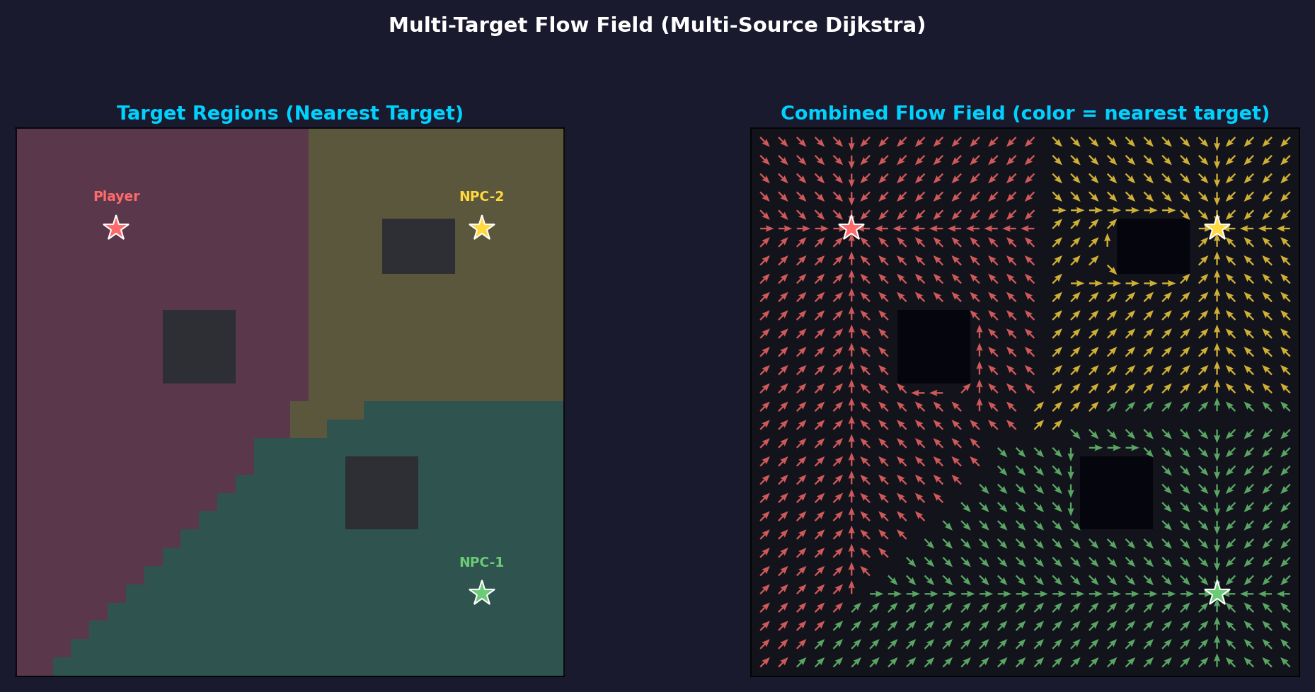Left: Territory partitioned by destination (based on nearest target). Right: Unified Flow Field — arrow color indicates the nearest destination.

---

Part 5: Flow Field — Generating Direction Vectors

From Integration Field to Flow Field

Once the Integration Field is complete, computing the Flow Field is straightforward. For each cell, simply record the direction toward the neighbor with the lowest cumulative cost:

For each cell:
  1. Compare Integration values of 8-directional neighbors
  2. Select the direction of the neighbor with the smallest value
  3. Normalize and store the direction vector

Example: Integration Field → Flow Field

Integration Field:          Flow Field (directions):

 4  3  2  3  4              ↘  ↓  ↓  ↓  ↙
 3  2  1  2  3              →  ↘  ↓  ↙  ←
 2  1  0  1  2              →  →  ●  ←  ←
 3  2  1  2  3              →  ↗  ↑  ↖  ←
 4  3  2  3  4              ↗  ↑  ↑  ↑  ↖

● is the destination (cost 0). All arrows naturally point toward the destination.

Normalized Direction Vectors

Each cell in the Flow Field stores a normalized 2D vector (x, y):

\[\vec{d} = \text{normalize}(\text{neighbor}\_\text{min} - \text{current})\]

By storing floating-point vectors rather than restricting to 8 discrete directions, Bilinear Interpolation can produce smooth movement at cell boundaries.

Why This Stage Is Perfect for Parallelization

Flow Field computation is completely independent per cell. Computing cell A’s direction does not depend on cell B’s result. Therefore:

• Parallelizable per cell with IJobParallelFor
• Burst compilation enables automatic SIMD vectorization
• Also implementable as a GPU compute shader

In contrast, the Integration Field (Dial’s Algorithm) has sequential dependencies and must run on a single thread. This is one of the reasons for separating the pipeline into stages.

---

Part 6: Agent Movement — O(1) Lookup

Basic Movement

Once the Flow Field is complete, the agent movement logic is extremely simple:

// Pseudocode
Vector2 worldPos = agent.position;
int cellX = (int)(worldPos.x / cellSize);
int cellY = (int)(worldPos.y / cellSize);
int index = cellY * gridWidth + cellX;

Vector2 direction = flowField[index];  // O(1) lookup
agent.velocity = direction * speed;

This cost remains constant no matter how many agents there are. The Flow Field computation is already done; agents just perform an array lookup.

Bilinear Interpolation

If directions change abruptly at cell boundaries, agents can zigzag. Bilinear interpolation solves this.

Based on the agent’s exact position, it computes a weighted average of the direction vectors from the 4 surrounding cells:

\[\vec{d}\_\text{interpolated} = (1-t_x)(1-t_y)\vec{d}\_{00} + t_x(1-t_y)\vec{d}\_{10} + (1-t_x)t_y\vec{d}\_{01} + t_x \cdot t_y \cdot \vec{d}\_{11}\]

Here \(t_x, t_y\) are the relative position within the cell (0–1).

Interpolation effect at cell boundaries:

No interpolation:         With interpolation:
 ↓  ↓  →  →              ↓  ↘  →  →
 ↓  ↓  →  →              ↓  ↘  ↗→ →
 ↓  ↓  →  →              ↓  ↘→ →  →

Agent trajectory:        Agent trajectory:
 ┃              ╲
 ┃               ╲
 ┗━━━━━            ╲━━━━
 (sharp turn)       (smooth curve)

With interpolation, thousands of agents moving simultaneously produce a natural flow.

---

Part 7: Performance Analysis — Why It Works in Real-Time Games

Memory Usage

Based on a 200×200 grid:

Field	Size per Cell	Total Size
Cost Field	1 byte	40 KB
Integration Field	2 bytes (ushort)	80 KB
Flow Field	8 bytes (float2)	320 KB
Total		440 KB

With A*, storing paths for 3,000 agents averaging 50 waypoints each: 3,000 × 50 × 8 bytes = 1.2 MB. Flow Field uses less memory as well.

Computation Time (Benchmark Reference)

200×200 grid, Unity Burst + Jobs:

Stage	Parallelization	Approx. Time
Cost Field	IJobParallelFor	~0.1ms
Integration Field (Dial’s)	IJob (single thread)	~0.5ms
Flow Field	IJobParallelFor	~0.1ms
Total		~0.7ms

And this only occurs when the destination moves. If you recompute at 0.5-second intervals, only 2 times/sec × 0.7ms = 1.4ms per second is spent on pathfinding.

Meanwhile, running A* 3,000 times takes tens of milliseconds even after optimization.

Real-World Profiling — 20,000 Agent Stress Test

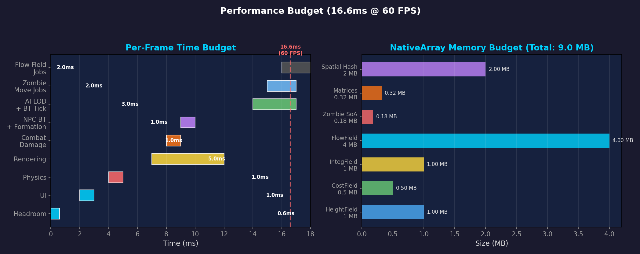Left: Per-system frame time budget (based on 16.6ms target). Right: NativeArray memory usage. Flow Field Jobs themselves are only 2ms — a fraction of the total.

In our actual project, rendering uses GPU Instancing + VAT animation. Stress testing with 20,000 agents yielded these results:

Metric	Value
p50 Frame Time	7.71ms
p90 Frame Time	8.34ms
p99 Frame Time	9.25ms
vs. 60fps Budget (16.67ms)	~54% headroom
Total Draw Calls	152
Triangles/Frame	41.2M

Even with 20,000 agents, p99 is 9.25ms — roughly half the 60fps budget. Pathfinding itself isn’t the bottleneck. Instead, agent sorting (NativeArray.Sort) was identified as consuming ~36.6% of frame time — which will be covered in a separate post.

Caching Strategy Summary

flowchart TD
    A{Did the terrain change?} -->|Yes| B[Recompute Cost Field]
    A -->|No| C{Did the destination move?}
    B --> D[Recompute Integration Field]
    C -->|Yes| D
    C -->|No| E[No recomputation — use cache]
    D --> F[Recompute Flow Field]
    F --> G[Agent movement: O_1 lookup]
    E --> G

    style E fill:#b7e8c4,stroke:#2e8b57,color:#333
    style G fill:#e8d5b7,stroke:#b8860b,color:#333

In most frames, agents use the cached Flow Field without any recomputation.

---

Summary: A* vs Flow Field

Aspect	A*	Flow Field
Computation Target	Path from start to goal	Direction vectors for entire space
Cost per Agent	\(O(E \log V)\)	\(O(1)\) (lookup only)
Total Cost for N Agents	\(O(N \cdot E \log V)\)	\(O(V)\) (independent of N)
Dynamic Environment Response	Recompute all agents	Recompute field once
Memory	Path stored per agent	3 fixed grids
Movement Quality	Individually optimal paths	Smooth crowd flow
Best Use Case	Few agents, diverse destinations	Many agents, shared destinations

Flow Field is not always superior. If you have 10 agents each heading to a different destination, A* is far more efficient. Flow Field shines in scenarios where “many agents share a small number of destinations” — zombie survival is exactly this case.

---

Upcoming Posts

This post covered the concepts behind Flow Field and its 3-stage pipeline. The next post will cover the practical optimizations applied when scaling from 3,000 to 10,000 agents using this Flow Field:

• 3K→10K Scaling — Burst SortJob, GPU Instancing + VAT, spatial hashing for separation steering, Tiered LOD, Frustum Culling
• Dial’s Algorithm Deep Dive — Circular bucket queue internals and implementation, 362-bucket system, real implementation patterns in Unity Jobs
• Multi-Goal & Layered Flow Field — Multiple destinations, layer separation strategies, cross-platform benchmarks

---

References

• Emerson, E. (2013). Crowd Pathfinding and Steering Using Flow Field Tiles. Game AI Pro.
• Pentheny, G. (2013). Efficient Crowd Simulation for Mobile Games. Game AI Pro.
• Dial, R.B. (1969). Algorithm 360: Shortest-path forest with topological ordering. Communications of the ACM, 12(11).